Which process runs next?
A CPU core runs one process at a time, and usually several are ready to run. The scheduler decides which one gets the CPU, and for how long. The context switch page shows how the kernel hands the CPU from one task to another; this page is about which task it hands it to, and what that choice costs each process.
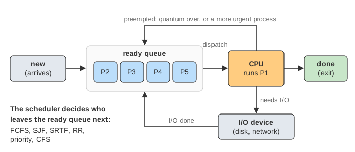
The animation runs the same few processes through seven policies, one time unit per step. Above: the processes and their counters, the ready queue (a list, or a red-black tree for CFS), the CPU and the I/O device. Below: the Gantt chart, one box per unit, and the results.
Terms
- A process alternates CPU bursts (computing) and I/O bursts (waiting for a disk, the network, the user). Only the CPU bursts compete for the CPU.
- Arrival: when it becomes ready for the first time. Completion: when its last burst ends.
- Turnaround = completion − arrival: how long the whole job took.
- Waiting = time spent in the ready queue = turnaround − CPU time (− I/O time, when there is I/O). The "waited" counters tick for every ready process.
- Response = first time on the CPU − arrival: how soon an interactive user sees a reaction.
- Throughput: processes finished per unit of time. Utilisation: the share of time the CPU is busy.
- Non-preemptive: a process keeps the CPU until its burst ends. Preemptive: the scheduler may take it away (a timer interrupt, or a more urgent process becoming ready). Every switch costs the dispatcher latency: saving and loading registers, and colder caches afterwards.
FCFS, SJF and SRTF
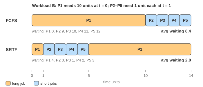
First-come, first-served is a FIFO queue. It is simple and starves nobody, but short jobs that arrive behind a long one wait for all of it: the convoy effect. On workload B (one 10-unit job, then four 1-unit jobs) the average waiting time is 8.4.
Shortest job first picks the process with the shortest next CPU burst. Among non-preemptive policies it gives the smallest average waiting time. The exchange argument: if a longer job runs just before a shorter one, swapping them makes the short one wait less by the long one's length and the long one wait more by only the short one's length, so the total drops. Its preemptive form, shortest remaining time first (SRTF), also preempts the running process when a newcomer needs less than it has left; it minimises average waiting among all these policies. On workload B, SJF cannot help (the long job is alone at t = 0), but SRTF drops the average waiting from 8.4 to 2.0.
The catch: nobody knows the length of the next burst. Real systems predict it from the past ones with an exponential average,
τ(n+1) = α · t(n) + (1 − α) · τ(n)          t(n) = the burst just measured, τ = the prediction

α = 1/2, τ(0) = 10, bursts 6, 4, 6, 4, 13:   predictions 10 → 8 → 6 → 6 → 5 → 9
A large α follows recent behaviour quickly; a small α remembers the long run. The animation gives SJF and SRTF the true burst lengths (an oracle).
Round Robin, priority and aging
Round Robin gives each process a quantum of CPU, then puts it at the tail of the queue. (When a process's quantum ends at the same moment as a new process arrives, this page puts the newcomer in the queue first, the common textbook convention.) Every process gets the CPU within a few quanta, so response time is short. But every job is stretched out, so turnaround can be worse than FCFS: on workload A, q = 2 cuts the average response from 5.8 (FCFS) to 2.2 but raises the average turnaround from 9.6 to 10.6. The quantum is a trade-off. As q grows, Round Robin turns into FCFS (q = 8 is FCFS on workload A: no burst is longer than 7). As q shrinks towards 0 it approaches "processor sharing", every process running at 1/n speed, paid for in context switches. A common rule of thumb: about 80% of CPU bursts should be shorter than the quantum.
Priority scheduling runs the most important process first (here, the smallest number). Its danger is starvation: as long as more important work keeps arriving, a low-priority process never runs. (A legend says that when MIT shut down its IBM 7094 in 1973, it found a low-priority job submitted in 1967 that had never run.) The cure is aging: the longer a process waits, the more important it becomes. On this page, every 4 units in the ready queue lower its number by 1, and it gets its own number back when it runs. Five processes cannot show real starvation, because the higher-priority work runs out; the demo shows P5's number dropping while it waits.
Priorities also meet locks: in priority inversion a high-priority task waits for a lock held by a low-priority one, which in turn cannot run because medium-priority tasks keep the CPU. Priority inheritance lends the holder the waiter's priority (see the lock side of it on the readers-writers page).
Multilevel feedback queues
Classic Unix and Windows schedulers used several queues, one per priority level, with Round Robin inside each. A process that uses up its whole quantum is moved down a level (it looks CPU-bound); one that blocks for I/O before its quantum ends stays up or moves up (it looks interactive). Interactive and I/O-bound programs get quick response without anybody declaring them interactive, and long CPU-bound jobs sink to the lower levels, which usually get longer quanta. Periodically every process is boosted back to the top, which is aging again.
Linux: from O(1) to CFS and EEVDF
Linux 2.6.0 used the O(1) scheduler, an array of priority queues with heuristics that guessed which tasks were interactive. In 2.6.23 (2007) it was replaced by the Completely Fair Scheduler, which has no quantum and no priority queues. Each task has a vruntime: the CPU time it has used, divided by its weight. The scheduler always runs the task with the smallest vruntime, so every task gets CPU in proportion to its weight.
- Weights and nice. Nice 0 has weight 1024, and each nice step changes the weight by about 1.25× (nice −5: 3121, nice 5: 335). vruntime grows by
time × 1024 / weight: a nice −5 task ages about 3× slower than a nice 0 one, so it gets about 3× the CPU when both want it. - The slice.
sched_latency(6 units here) is shared among the runnable tasks by weight: a task's slice islatency × weight / total weight, but at least the minimum granularity (1 unit here). - New and waking tasks. A new task starts at
min_vruntime, the smallest vruntime in the queue; a task waking from I/O is placed atmax(own vruntime, min_vruntime − latency/2). The small credit lets it run soon, but it cannot hoard the CPU with credit saved while asleep. It preempts the running task only when its vruntime is lower by more than the wake-up granularity (1 unit here). - Why a red-black tree. The runnable tasks are kept in a red-black tree ordered by vruntime: insert and remove are O(log n), and the leftmost node (the next task) is cached, so picking it is O(1). A red-black tree rather than an AVL tree, because it bounds the rotations per update (see AVL vs red-black). The running task is taken out of the tree while it runs, as here.
- EEVDF. Since Linux 6.6 (2023) the fair class uses Earliest Eligible Virtual Deadline First. It keeps vruntime and the red-black tree, but adds a lag (how much CPU a task is owed) and a virtual deadline per task; among the tasks that are owed CPU it picks the earliest deadline. That gives latency-sensitive tasks shorter slices without heuristics. The animation shows classic CFS; the difference is not animated.
- Other classes. Above the fair class are the real-time classes
SCHED_FIFOandSCHED_RR(fixed priorities 1–99, FCFS or Round Robin within a priority) and, above those,SCHED_DEADLINE(earliest deadline first with a runtime budget per period). A runnable real-time task always runs before any normal task.
More than one CPU
A real machine has many cores, and each has its own run queue (in Linux, its own red-black tree). A load balancer moves tasks from busy queues to idle ones, but not too eagerly: a task that moves loses its warm caches, so schedulers prefer affinity (keeping a task where it ran before), and programs can pin tasks to cores with taskset or sched_setaffinity. The animation has one CPU; Concurrency vs Parallelism runs the same threads on 1, 2 and 4 cores.
How to see it on a real system
nice -n 5 ./job                  # start with nice 5;   renice -n -5 -p <pid>  to change it
chrt -f 50 ./job                 # SCHED_FIFO at priority 50;   chrt -p <pid>  shows the policy
cat /proc/<pid>/sched            # se.vruntime, se.sum_exec_runtime, nr_switches, ...
perf sched record ./job; perf sched latency     # how long each task waited to run
schedtool <pid>                  # policy, priority and affinity at a glance
What the animation leaves out
- One CPU, whole time units, and the scheduler only acts at unit boundaries (a real kernel also switches the moment a task blocks or a more urgent one wakes).
- SJF and SRTF know every burst length in advance (see the prediction above).
- CFS is simplified: no
START_DEBIT, no task groups, no per-CPU queues, slices checked once per unit; Linux 6.6+ uses EEVDF, which is described but not animated. - Context switches take no time in the Gantt chart; the optional switch cost only adds dispatches × cost to the results.
- I/O is one FCFS device with fixed durations.