Disjoint Sets Visualization | Disjoint Sets Animation

Some applications involve grouping $n$ distinct objects into a collection of disjoint sets. Two important operations are then finding which set a given object belongs to and uniting the two sets.

A disjoint set data structure maintains a collection $S = {S_{1}, S_{2}, \dots, S_{k}}$ of disjoint dynamic sets. Each set is identified by a representative, which usually is a member in the set.

1 Operations on Sets

Let $x$ be an object. We wish to support the following operations.

Make-Set( $x$ ) creates a new set whose only member is pointed by $x$ ; Note that $x$ is not in the other sets.
Union( $x, y$ ) unites two dynamic sets containing objects $x$ and $y$ , say $S_{x}$ and $S_{y}$ , into a new set that $S_{x} \cup S_{y}$ , assuming that $S_{x} \cap S_{y} = \emptyset$ ;
Find-Set( $x$ ) returns a pointer to the representative of the set containing $x$ .
Insert( $a, S$ ) inserts an object $a$ to $S$ , and returns $S \cup {a}$ .
Delete( $a, S$ ) deletes an object $a$ from $S$ , and returns $S - {a}$ .
Split( $a, S$ ) partitions the objects of $S$ into two sets $S_{1}$ and $S_{2}$ such that $S_{1} = {b | b \leq a & b \in S}$ , and $S_{2} = S - S_{1}$ .
Minimum( $S$ ) returns the minimum object in $S$ .

2 Applications of Disjoint-set Data Structures

Here we show two application examples.

Connected components (CCs)
Minimum Spanning Trees (MSTs)

2.1 Algorithm for Connected Components

Connected-Components  $(G)$ 
 1    for each  $v \in V$ 
 2             do  Make-Set  $(v)$ 
 3    for every edge  $(u, v) \in E$ 
 4             do if  Find-Set  $(u)$   $\neq$  Find-Set  $(v)$ 
 5                         then  Union  $(u, v)$

Same-Components  $(u, v)$ 
 1    if  Find-Set  $(u)$   $=$  Find-Set  $(v)$ 
 2          then return TRUE
 3    return FALSE

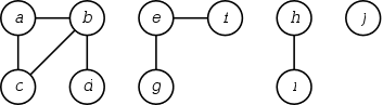
Undirected graph on vertices a to j with four connected components: a, b, c, d joined by edges; e, f, g; h, i; and j on its own

Figure 1: A graph with four connected components: ${a, b, c, d}$ , ${e, f, g}$ , ${h, i}$ , and ${j}$ .

Edge processed	Collection of disjoint sets
initial sets	${a}$	${b}$	${c}$	${d}$	${e}$	${f}$	${g}$	${h}$	${i}$	${j}$
$(b, d)$	${a}$	${b, d}$	${c}$		${e}$	${f}$	${g}$	${h}$	${i}$	${j}$
$(e, g)$	${a}$	${b, d}$	${c}$		${e, g}$	${f}$		${h}$	${i}$	${j}$
$(a, c)$	${a, c}$	${b, d}$			${e, g}$	${f}$		${h}$	${i}$	${j}$
$(h, i)$	${a, c}$	${b, d}$			${e, g}$	${f}$		${h, i}$		${j}$
$(a, b)$	${a, b, c, d}$				${e, g}$	${f}$		${h, i}$		${j}$
$(e, f)$	${a, b, c, d}$				${e, f, g}$			${h, i}$		${j}$
$(b, c)$	${a, b, c, d}$				${e, f, g}$			${h, i}$		${j}$

Table 1: This table shows the state of the collection of disjoint sets as each edge is processed. The processed edge is listed on the left and the rest of the columns show the state of the collection.

3 The Disjoint Set Representation

3.1 The Linked-list Representation

A set can be represented by a linked list. In this representation, each node has a pointer to the next node and a pointer to the first node.

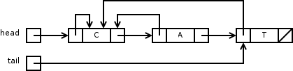
A set stored as a linked list c, a, t: head points to the first node and tail to the last; every node has a next pointer and a pointer back to the first node

Figure 2: Linked-list representation. Each disjoint set can be represented by a linked-list. Each node has a pointer to the head node and a pointer to the next node.

Consider the following operation sequence:

Make-Set $(x_{1})$ ,
Make-Set $(x_{2})$ ,
$:$ ,
Make-Set $(x_{n - 1})$ ,
Make-Set $(x_{n})$ ,
Union $(x_{1}, x_{2})$ ,
Union $(x_{2}, x_{3})$ ,
$:$ ,
Union $(x_{n - 1}, x_{n})$ .

What's the total time complexity of the above operations?

A weighted-union heuristic: Assume that the representative of each set maintains the number of objects in the set, and always merge the smaller list to the larger list, then

Theorem: Using the linked list representation of disjoint sets and the weighted-union heuristic, a sequence of $m$ Make-Set, Union, and Find_Set operations, $n$ of which are Make-Set, takes $O (m + n \log n)$ time.

Hint: observe that for any $k \leq n$ , after $x$ 's representative pointer has been updated $⌈ \log k ⌉$ times, the resulting set containing $x$ must have at least $k$ members.

4 Disjoint Set Forests

A faster implementation of disjoint sets is through the rooted trees, with each node containing one member and each tree representing one set. Each member in the tree has only one parent.

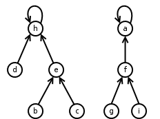
Two rooted trees with parent pointers: root h with children d and e, e with children b and c; root a with child f, f with children g and i; each root points to itself

Figure 3: Rooted tree representation of disjoint sets. Each tree has a "representative" $h$ for the left tree and $a$ for the right tree.

4.1 The Heuristics for Disjoint Set Operations

union by rank.
path compression

The idea of union by rank is to make the root of the tree with fewer nodes point to the root of the tree with more nodes. Rather than explicitly keeping track of the size of the subtree rooted at each node, for each node we maintain a rank that approximates the logarithm of the subtree size and is also an upper bound on the height of the node.

Time complexity: $O (m \log n)$ , assuming that there are $m$ union operations.

Path compression is quite simple and very effective. We use this approach during Find-Set operations to make each node on the path point directly to the root. Path compression does not change any ranks.

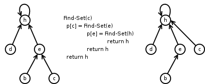
Path compression: before, c points to e and e to the root h; the recursive calls Find-Set(c), Find-Set(e), Find-Set(h) return h; after, c and e both point directly to h

Figure 4: Path compression takes place during the Find-Set operation. This works by recursing from the given input node up to the root of the tree, forming a path. Then the root is returned and assigned as the parent for each node in path. The parent of $c$ after Find-Set $(c)$ is $h$ .

Time complexity: $Θ (f \log_{1 + f / n)} n)$ if $f \geq n$ and $Θ (n + f \log n)$ otherwise, assume that there are $n$ Make-Set operations and $f$ Find-Set operations.

Make-Set  $(x)$ 
 1      $p [x]$    $\leftarrow$    $x$ 
 2      $rank [x]$    $\leftarrow$    $0$

Find-Set  $(x)$ 
 1    if   $x \neq p [x]$ 
 2          then   $p [x]$    $\leftarrow$   Find-Set  $(p [x])$ 
 3    return   $p [x]$

Union  $(x, y)$ 
 1     Link( Find-Set  $(x)$ , Find-Set  $(y)$ )

Link  $(x, y)$ 
 1    if   $rank [x] > rank [y]$ 
 2          then   $p [y]$    $\leftarrow$    $x$ 
 3          else    $p [x]$    $\leftarrow$    $y$ 
 4                      if   $rank [x] = rank [y]$ 
 5                            then   $rank [y]$    $\leftarrow$    $rank [y] + 1$

where $rank [x]$ is the height of $x$ in the tree. If both of the above methods are used together, the time complexity is $O (m α (m, n))$ .

The Rank properties

$rank [x] \leq rank [p [x]]$
for any tree root $x$ , $size (x) \geq 2^{rank [x]}$ (Link operation)
for any integer $r$ , there are at most $n / 2^{r}$ nodes of rank $r$
each node has rank at most $⌊ \log n ⌋$ , assuming there are at $n$ objects involved.

Where union-find is used

Union-find is a small structure with an unusually wide reach, because "these two things are now in the same group, and stay there" describes a great many problems. With union by rank and path compression, a sequence of m operations costs O(m α(n)), where α is the inverse Ackermann function — below 5 for any n that will ever be stored, so each operation is effectively constant time.

Minimum spanning trees. Kruskal's algorithm is union-find plus a sort: walk the edges cheapest first, and take an edge exactly when its endpoints are still in different sets. Without this structure the cycle test would dominate the running time.
Connectivity. Which machines can reach each other, which pixels belong to the same blob, whether a network is still in one piece after a link is added. Union-find answers this as the edges arrive, without re-running a search.
Image segmentation. The Felzenszwalb-Huttenlocher segmentation algorithm is essentially Kruskal over a pixel grid, merging regions while a similarity predicate holds.
Compilers and type systems. Hindley-Milner type inference unifies type variables by merging equivalence classes. Register allocators coalesce registers the same way, and congruence closure in SMT solvers merges terms known to be equal.
Equivalence and closure problems generally: minimising a finite automaton by merging indistinguishable states, grouping records that refer to the same real entity, maintaining equivalence classes in a constraint solver.
Percolation and physics simulation, where the question is whether a cluster has grown across the whole grid, and the Hoshen-Kopelman labelling algorithm is union-find in disguise.
Maze generation, knocking down walls between cells that are not yet connected, and offline lowest common ancestor queries via Tarjan's algorithm.

The one thing it cannot do is undo. Union-find merges sets and never splits them, so a problem with edge deletions needs something else — which is why algorithms are often restructured to process deletions backwards in time, turning them into insertions.

References

Disjoint-set data structure (Wikipedia)

Sedgewick and Wayne, Algorithms 4th ed.: Union-Find