The idea: centres that are real points
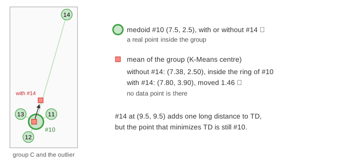
K-Means puts each centre at the mean of its points. A mean is usually not a data point, and one far-away point can pull it a long way. k-medoids chooses k of the data points themselves as centres. Such a centre is a medoid: the point of its group with the smallest total distance to the others. Every point joins its nearest medoid.
The cost: total distance TD
k-medoids minimizes the total distance TD: the sum, over all points, of the distance to the nearest medoid. The distances are plain (here Euclidean), not squared as in the K-Means SSE. Squaring makes a far point count much more, so it is one reason K-Means is more sensitive to outliers. Because only distances between data points are needed, k-medoids also works with any dissimilarity: Manhattan distance, edit distance between strings, or a ready-made distance matrix.
On the canvas a thin line joins each point to its medoid; TD is the total length of these lines.
PAM: BUILD, then SWAP
PAM (Partitioning Around Medoids, Kaufman and Rousseeuw) has two phases:
- BUILD: pick the point that gives the lowest TD as the only medoid; then, k − 1 more times, add the point that lowers TD the most.
- SWAP: for every medoid m and every non-medoid o, compute TD if o replaces m. That is k × (n − k) pairs, 3 × 10 = 30 on the page. If the best pair lowers TD, swap it and repeat. If no pair lowers TD, stop.
The panel lists, for each medoid, the best non-medoid to swap it with and the TD that would give; the green row is the swap that is made. (Demo 2: BUILD, then SWAP: BUILD picks #5, #10 and #6, TD = 14.64; one swap, #5 out and #1 in, gives TD = 11.70, the best possible for k = 3.)
The start matters: local optima
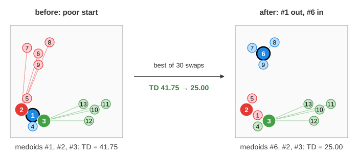
SWAP only accepts a trade that lowers TD, so it always stops, but it can stop at a local optimum, where no single swap helps though a better set of medoids exists.
| Run | TD after each step | Result |
|---|---|---|
| k = 3, poor start #1 #2 #3 (Demo 1) | 41.75 → 25.00 → 13.16 → 11.70 | 3 swaps, best possible |
| k = 3, BUILD (Demo 2) | 14.64 → 11.70 | 1 swap, best possible |
| k = 2, poor start #1 #2 (Demo 3) | 46.48 → 30.08 → 28.62 | stops; the best is 28.27 (BUILD finds it) |
BUILD costs more than a random start, but it usually starts close to the answer, so few swaps follow. Some libraries start with k-medoids++ (random seeding as in k-means++) instead and accept the risk.
Outliers: medoid vs mean
Add #14 at (9.5, 9.5) and run PAM with k = 3: it joins group C, but the medoid of C stays #10 (7.5, 2.5). The K-Means button runs Lloyd's algorithm from the same medoids. The mean of C moves from (7.38, 2.50) to (7.80, 3.90), 1.46 away, to a place where there is no data. (Demo 4: an outlier pulls the mean)
| K-Means | k-medoids (PAM) | |
|---|---|---|
| centre | mean, any point in space | one of the data points |
| cost | sum of squared distances (SSE) | sum of distances (TD) |
| one outlier | pulls the mean toward it | adds one distance; the medoid stays |
| distance | Euclidean (the mean needs coordinates) | any dissimilarity |
| cost per round | O(nk) | O(k(n − k)²) for a PAM SWAP round |
The silhouette of one point
A clustering is good when each point is close to its own cluster and far from the others. The silhouette measures this per point i:
- a(i): the mean distance from i to the other points of its own cluster.
- b(i): the mean distance from i to the points of each other cluster; take the smallest (the nearest other cluster).
- s(i) = (b − a) / max(a, b), between −1 and 1.
s near 1: well inside its cluster. Near 0: on the border between two clusters. Below 0: on average closer to another cluster, so probably in the wrong one. A point alone in its cluster has no a(i); it gets s = 0.
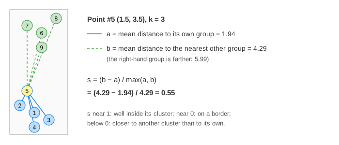
The Silhouette button first works through the point with the lowest s, then draws all bars, grouped by cluster, and the average silhouette s̄ as a black line. (Demo 5: k = 3 gives s̄ = 0.70; the lowest is #5 with 0.55.) With the outlier, #14 gets s = −0.01 for k = 3: it is about as far from its own group C as from group B.
Choosing k with the average silhouette
TD always falls when k grows (one more medoid can only bring points closer), so the lowest TD would always pick the largest k. The average silhouette does not: too few clusters make a(i) large, too many split a group so that b(i) becomes small. Pick the k with the highest s̄. (Demo 6: choose k)
| k | TD | average s |
|---|---|---|
| 2 | 28.27 | 0.49 |
| 3 | 11.70 | 0.70 ✓ highest |
| 4 | 10.12 | 0.58 |
With the outlier and k = 4, PAM gives #14 a medoid of its own (TD = 11.70); #14 is then alone and gets s = 0, and s̄ = 0.65. (Demo 7) Kaufman and Rousseeuw's rough guide: s̄ above 0.70 means a strong structure, 0.51–0.70 a reasonable one, 0.26–0.50 a weak one, and 0.25 or less no real structure.
The silhouette works for any clustering, not only k-medoids: it can also score K-Means (next to its elbow plot), a cut of a dendrogram or DBSCAN (leaving the noise out). For soft clusters with probabilities, see K-Means vs Gaussian mixtures.
Cost and faster variants
- A plain PAM SWAP round tries k(n − k) pairs and each costs O(n), so O(k(n − k)²) per round: fine for thousands of points, too slow for millions.
- CLARA runs PAM on several random samples and keeps the medoids with the lowest TD on all the data; CLARANS tries random swaps instead of all of them.
- FasterPAM (Schubert and Rousseeuw) finds the same kind of answer about O(k) times faster by sharing work between pairs and taking the first good swap.
- The silhouette needs all pairwise distances: O(n²).
See also The EM Algorithm, Step by Step for soft clustering with a mixture of Gaussians fitted by EM.
What the page leaves out
The data has 13 or 14 points in 2-D, so every swap and every distance can be shown. The page uses Euclidean distance only, and PAM as first described (best swap per round); it does not run CLARA, CLARANS or FasterPAM, and skips the "alternating" k-medoids (a K-Means-like loop) that is faster but finds worse answers. Other ways to choose k (the gap statistic, the elbow on TD) and the silhouette plot of very large data sets are only mentioned.