The idea: guess the next word from the last one
A language model gives every sentence a probability. Good sentences get a high one,
odd ones a low one. An n-gram model does this with plain counting. A bigram
model (n = 2) looks only at the previous word: how often is like followed by ham
in the training text?
The canvas trains on three short sentences: I like ham, I like eggs and
you like ham and eggs. Before counting, each sentence gets a start mark <s>
and an end mark </s>. The model then also learns which words start a sentence and which
end one.
Counting bigrams
Slide a window of two words along each sentence and add 1 to the cell (previous word, next word). The three
sentences hold 14 pairs, one for every predicted token (</s> is predicted,
<s> is not). The row total c(prev) says how often a word is followed by
anything. The column total c(next) is the plain word count, the unigram
count. (Demo 1: count bigrams from the corpus)
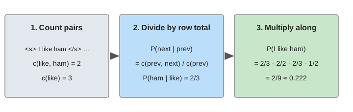
Dividing each cell by its row total gives the maximum likelihood estimate:
P(next | prev) = c(prev, next) / c(prev)
P(ham | like)  = 2 / 3        P(I | <s>) = 2 / 3        P(</s> | eggs) = 2 / 2
The probability of a sentence
The chain rule writes P(w1 … wn) as P(w1) · P(w2 | w1) · P(w3 | w1 w2) · … The bigram model makes one simplifying guess, the Markov assumption: each word depends only on the word just before it. So a sentence's probability is just the product of its bigram probabilities.
P(<s> I like ham </s>) = P(I|<s>) · P(like|I) · P(ham|like) · P(</s>|ham)
= 2/3 · 2/2 · 2/3 · 1/2 = 2/9 ≈ 0.222(Demo 2: score a training sentence) The model also scores sentences it never saw.
you like eggs is not in the corpus, but each of its pairs is, so it gets 1/3 · 1/1 · 1/3 · 2/2
= 1/9. (Demo 3: a new sentence still scores) Real systems add log probabilities
instead of multiplying, because a product of hundreds of small numbers underflows to 0.
One zero count kills the sentence
I like eggs and ham is a normal sentence. But the pair (eggs, and) never occurs in the corpus (nor does (and, ham)),
so P(and | eggs) = 0/2 = 0, and the whole product is 0. The model calls the sentence impossible. Any real
corpus is too small to hold every reasonable pair, so this happens all the time.
(Demo 4: one zero count kills the sentence) Smoothing moves a little probability
from seen pairs to unseen ones.
Add-one (Laplace) smoothing
Pretend every pair was seen once more than it was. With V = 7 possible next words each row total grows by 7:
P(next | prev) = (c(prev, next) + 1) / (c(prev) + 7)
P(and | eggs)  = (0 + 1) / (2 + 7) = 1/9
Now I like eggs and ham gets 1/16200 ≈ 0.0000617. But add-one is crude. It gives the same
extra count to every one of the 49 cells, and most of them are nonsense pairs. The probability has to come
from somewhere: the training sentence I like ham falls from 2/9 ≈ 0.222 to 1/150 ≈ 0.00667.
(Demo 5: add-one smoothing) The same idea is used for word counts in the
Naive Bayes spam filter.
Backoff: ask the unigram model
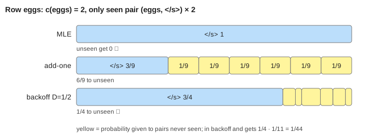
Backoff is smarter about where the freed probability goes. Take a small discount
D = 1/2 from every seen count. In row eggs the only seen pair is (eggs, </s>) with count 2,
so P(</s> | eggs) = (2 − 1/2) / 2 = 3/4, and 1/4 is freed. The unseen words share that 1/4 in
proportion to how common they are on their own, c(next). and occurs once out of the 11 counts of
the unseen words, so P(and | eggs) = 1/4 · 1/11 = 1/44. Every row still sums to 1.
(Demo 6: backoff to the unigram)
This is the idea behind Katz backoff and absolute discounting. The best classic method, Kneser-Ney, adds one more trick: it backs off to how many different words a word follows, not to its raw count.
Perplexity: one number to compare models
To compare models, score text they did not train on. Perplexity is the probability of the test text, turned into a per-word number:
PP = P(test) ^ (−1/N) N = number of predicted tokens (here 4 + 6 = 10)A perplexity of 4.48 means the model is, on average, as unsure as if it picked among about 4.5 equally
likely words at every position. Lower is better. It is the same as 2 raised to the cross-entropy
in bits per word (log2 4.48 ≈ 2.16 bits). The test set is you like eggs and
I like eggs and ham. (Demo 7: perplexity, four models compared)
| Model | P(test) | Perplexity |
|---|---|---|
| Unigram (ignores the previous word) | ≈ 0.0000000045 | 6.84 |
| Bigram, MLE (no smoothing) | 0 | ∞ |
| Bigram, add-one | 1/300 · 1/16200 | 4.66 |
| Bigram, backoff D = 1/2 | 1/96 · 1/33792 | 4.48 |
On its own training text the unsmoothed bigram would look best, because it memorised the counts. That is why models are always compared on held-out text.
Bigger n, bigger data
A trigram model looks at two previous words, P(w | u v) = c(u, v, w) / c(u, v). Longer contexts predict better but make the zero problem much worse: most 4-word sequences never occur even in billions of words. Classic systems used 3- to 5-grams with Kneser-Ney smoothing, trained on huge corpora. For very large data, the simple "stupid backoff" (multiply by 0.4 and use the shorter context) works well enough, though its scores are not true probabilities.
A bigram model is a Markov chain whose states are words, with transition probabilities learned from counts. Neural models drop the fixed window: Word2Vec learns word vectors from the same kind of context counts, and a large language model predicts the next BPE token from thousands of previous ones. It is still trained and measured by the same loss, the cross-entropy of the next token, and its text is produced by decoding strategies.
See also Part-of-Speech Tagging with an HMM, which counts bigrams of tags instead of words and shows how one unseen word breaks a tagger built on raw counts.
What the page leaves out
Trigrams and longer contexts, Good-Turing estimates, Kneser-Ney and interpolation (mixing all orders with
weights), unknown words and the <UNK> token, tuning D on held-out data, and storing
billions of n-grams compactly. The corpus has 3 sentences; real models count over billions of words.