The idea: an RDD is a recipe, not data
In Apache Spark an RDD (resilient distributed dataset) is a collection cut into partitions that live on different machines. But an RDD object in your program holds no records. It holds a recipe: which RDD it comes from and which function to apply. The chain of recipes back to the input file is the RDD's lineage. Spark computes real records only when the program asks for a result, and it can compute any partition again from its lineage if the copy is lost.
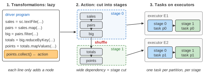
The page runs a five-line program on a tiny file of sales, product,amount, stored in two HDFS blocks. There is one driver (your program) and two executors, E1 and E2, which run the tasks. Every RDD has 2 partitions; partition 0 is computed on E1 and partition 1 on E2.
| RDD | Line of the program | Partition 0 | Partition 1 |
|---|---|---|---|
| sales | sc.textFile("sales.csv", 2) | tea,3 milk,5 tea,4 | jam,2 milk,6 tea,1 |
| pairs | sales.map(parse) | (tea,3) (milk,5) (tea,4) | (jam,2) (milk,6) (tea,1) |
| big | pairs.filter(v >= 2) | (tea,3) (milk,5) (tea,4) | (jam,2) (milk,6) |
| totals | big.reduceByKey(_ + _) | (tea,7) (jam,2) | (milk,11) |
| points | totals.mapValues(_ * 10) | (tea,70) (jam,20) | (milk,110) |
On the canvas a box is one partition. A white box that says (no data) is only a recipe. Orange means a task is computing it now, blue means it is cached in executor memory, green is a shuffle file on an executor's disk, and red was lost with its executor.
Transformations are lazy, actions run jobs
A transformation makes a new RDD from an old one. Calling it does no work: the driver only adds a node and its arrows to the lineage graph. In Demo 1 all five lines run and the counters still show 0 jobs, 0 tasks and 0 partitions computed. The file has not even been opened.
An action returns a value to the driver or writes output, so it needs real records. Each action starts one job. Being lazy lets Spark see the whole chain before it runs anything, so it can put several steps into one task and skip work that no action needs.
| Kind | Examples | What the call does |
|---|---|---|
| Transformation, narrow | map, filter, flatMap, mapValues, union | adds an RDD to the lineage; returns at once |
| Transformation, wide | reduceByKey, groupByKey, join, repartition, sortByKey | adds an RDD and a shuffle to the lineage; returns at once |
| Action | collect, count, take, reduce, saveAsTextFile | starts a job and waits for its result |
Narrow and wide dependencies
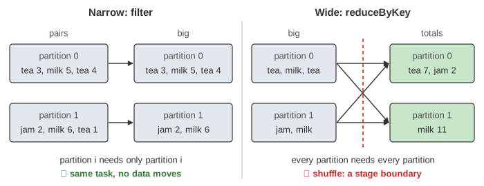
A dependency is narrow when each partition of the parent is used by at most one partition of the child. map and filter are narrow: partition 1 of big needs only partition 1 of pairs. The work stays on one executor, and no record moves.
A dependency is wide when a child partition needs records from many parent partitions. reduceByKey must add up all amounts of tea, and tea is in both partitions of big. So Spark does a shuffle: every map-side task writes its records to a shuffle file on local disk, grouped by target partition (hash(key) mod 2), and every task on the other side fetches its share from each file. On the page the hash is the sum of the letter codes, so tea and jam go to partition 0 and milk goes to partition 1. reduceByKey also adds up equal keys before writing, so partition 0 writes (tea,7), not two tea records: 4 records cross the shuffle instead of 5. MapReduce shows this combine step, the partitioner and the sort in detail.
Stages and tasks
When an action is called, the driver's DAG scheduler walks the lineage backwards from the target RDD. It keeps going through narrow dependencies and cuts at every wide one. Each piece is a stage. A stage runs as one task per partition, and a task runs the whole narrow chain of its stage for its own partition, record after record, without storing the steps in between.
In Demo 2, points.collect() gives two stages. Stage 0 is a shuffle map stage: 2 tasks read their block, run sales → pairs → big and write shuffle files. Stage 1 is the result stage: 2 tasks read the shuffle, run totals → points and send their records to the driver. That is 4 tasks and 10 RDD partitions computed (5 RDDs × 2 partitions). Stage 1 cannot start before stage 0 has finished, because it needs every shuffle file. The stages form a graph with no cycles, and Spark runs them in an order where parents come first, the same idea as a topological sort.
In Demo 3 the program stops after big. big.collect() meets only narrow dependencies, so the job has one stage, 2 tasks and no shuffle at all.
A second action, and cache()
When a job ends, the partitions it computed are gone: they were only streams of records passing through the tasks. So a second action starts again from the lineage. In Demo 4, points.count() after points.collect() computes totals and points a second time. It does not rerun the first stage, but only because the shuffle files are still on the executors' disks; the Spark UI shows that stage as skipped.
cache() marks an RDD so that executors keep its partitions in memory when they are first computed (it is short for persist(MEMORY_ONLY)). It is lazy too: nothing is stored until an action runs. In Demo 5 the first job fills two blue blocks, and the second job finds both. It still runs 2 tasks, but they compute nothing.
Second action, points.count() | Stage 2 (map) | Stage 3 (result) | RDD partitions computed | Cache hits |
|---|---|---|---|---|
| no cache (Demo 4) | skipped | 2 tasks | 4 | 0 |
points.cache() (Demo 5) | skipped | 2 tasks | 0 | 2 |
| cache, then E2 is lost (Demo 6) | 1 task | 2 tasks | 5 | 1 |
Cache an RDD that is used by more than one action and is costly to compute. Caching everything wastes memory: when memory runs out, Spark drops old blocks and computes them again from lineage when needed.
A lost partition is recomputed from lineage
Spark does not copy RDD partitions to other machines to survive a crash. It keeps the lineage in the driver, which is small, and recomputes. In Demo 6 executor E2 dies after the first job. Two things die with it: the cached block points[1] and the shuffle file that map task 1 wrote. The block points[0] and the other shuffle file, on E1, are fine.
The next action needs points[1] again. The DAG scheduler follows its lineage back: points[1] needs totals[1], which needs both shuffle files, and one is missing. So the map stage runs again with 1 task, for partition 1 only: it reads block 1 from HDFS again (HDFS keeps replicas, see HDFS read and write) and rewrites the file. Then the result stage computes totals[1] and points[1], while partition 0 is a cache hit. Only 5 of the 10 RDD partitions are computed again, and the answer is the same, 3.
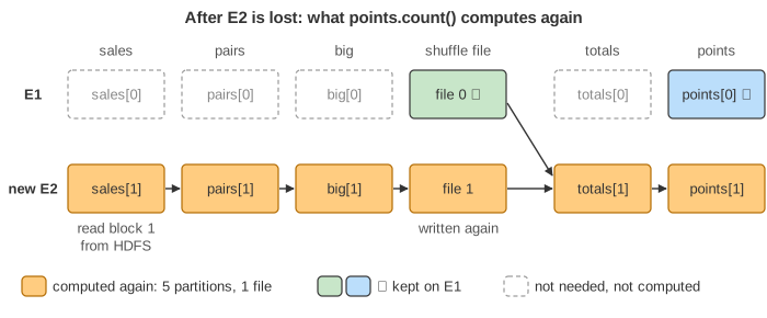
This works because transformations are deterministic and the input is still there. Recomputing is cheap when the lineage is short and narrow, and costly when it is long or crosses several shuffles.
See also MapReduce, where every job is one map stage and one reduce stage with output written to HDFS, and Range vs Hash Partitioning for how keys are assigned to partitions.
See also Stream Windows and Watermarks for Spark Structured Streaming's windows, withWatermark and late data on a stream instead of a fixed batch.
See also Lambda vs Kappa architecture, where a Spark batch job recomputes the batch view and a stream job keeps the realtime view.
What the page leaves out
Real jobs have hundreds of partitions and many executors, and a partition can run on any executor; the page pins partition 0 to E1 and partition 1 to E2. Inside a task Spark pipes one record at a time through the whole narrow chain; the page shows one RDD per step. The driver here learns about the lost executor at once; in practice a task often finds out through a failed shuffle fetch, and the stages are then resubmitted. An external shuffle service can keep shuffle files alive when an executor dies. Left out as well: other storage levels (MEMORY_AND_DISK), checkpoint(), which saves an RDD to HDFS and cuts its lineage, unpersist(), task retries and speculation, data locality, broadcast variables and accumulators, and the DataFrame API, whose Catalyst optimizer rewrites the plan before it becomes RDDs. Simplifications: the hash is the sum of the letter codes, and results are shown in partition order.