The idea: blame flows backwards
To train a network with gradient descent we need ∂L/∂θ for every parameter θ: how much the loss changes when θ is nudged. Backpropagation computes all of them in one pass that goes from the loss back to the inputs, applying the chain rule at each neuron and reusing the values saved during the forward pass.
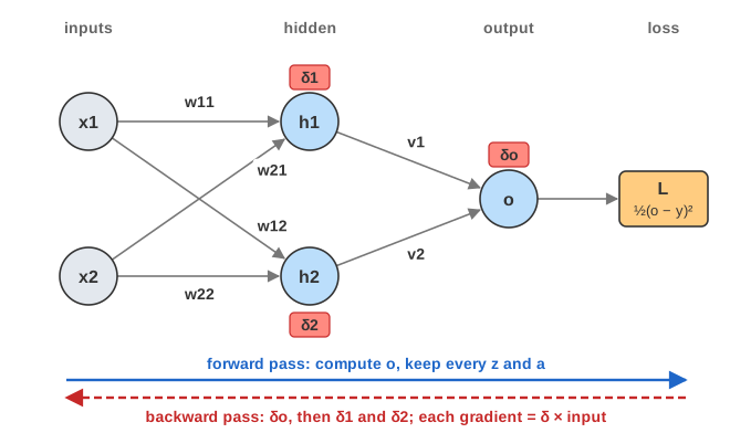
The page uses the smallest network that can learn XOR: 2 inputs, 2 hidden neurons, 1 output — 9 parameters. XOR is not linearly separable, so the hidden layer is needed.
A neuron: weighted sum and activation
Each neuron is drawn as two boxes. The first holds the weighted sum z = Σ w·x + b, the second the activation a = f(z). The hidden layer uses sigmoid σ(z) = 1/(1 + e−z) or ReLU(z) = max(0, z); the output always uses a sigmoid, so o is between 0 and 1.
Forward pass
z1 = w11·x1 + w21·x2 + b1, a1 = f(z1) (same for h2), then z = v1·a1 + v2·a2 + c and o = σ(z). Every intermediate value (blue) is kept: the backward pass needs them. (Demo 1: one sample — forward, backward, update)
The loss
For one sample, L = ½(o − y)². The ½ cancels when differentiating: ∂L/∂o = o − y. Classifiers usually use cross-entropy instead; with a sigmoid output it makes the output delta simply o − y.
The chain rule
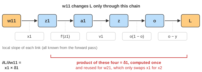
w11 changes L only through the chain z1 → a1 → z → o → L. The derivative of a chain is the product of the local derivatives: ∂L/∂w11 = (o − y) · o(1 − o) · v1 · f'(z1) · x1. Each factor is known locally. (Demo 2: the chain rule along one path)
Backward pass: the four equations
Define a neuron's delta δ = ∂L/∂z (red). Then:
| what | formula | in words |
|---|---|---|
| output delta | δo = (o − y) · σ'(z) | error times the output's slope |
| hidden delta | δj = vj · δo · f'(zj) | the delta above, sent back along the weight, times this neuron's slope |
| weight gradient | ∂L/∂w = δ(target neuron) · a(source) | blame at the end × value that went in |
| bias gradient | ∂L/∂b = δ | the bias input is always 1 |
In a bigger network with a layer's weights as a matrix W: δ(l) = (W(l+1))ᵀ δ(l+1) ⊙ f'(z(l)) and ∂L/∂W(l) = δ(l) (a(l−1))ᵀ.
Why it is cheap
The product for ∂L/∂w11 and the one for ∂L/∂w21 share every factor except the last. Backprop computes the shared part once
(as δ1) and reuses it. So all gradients cost about one extra pass, whatever the number of parameters. This is
reverse-mode automatic differentiation, what PyTorch's loss.backward() and JAX's grad do.
Updating the weights
θ ← θ − η·∂L/∂θ for all 9 parameters. Updating after every sample is stochastic gradient descent; one epoch is one pass over the 4 samples. With the preset weights and η = 2, the loss sits on a plateau around 0.5 for ~200 epochs, then drops, and XOR is solved after 523 epochs. (Demo 3) η = 0.1 is still on the plateau after 1000 epochs; η = 50 overshoots and never settles. (Demo 4) See Gradient Descent for the learning rate in detail.
Activation derivatives
| activation | f(z) | f'(z) | largest f' |
|---|---|---|---|
| sigmoid | 1 / (1 + e−z) | σ(z)(1 − σ(z)) | 0.25 at z = 0 |
| tanh | (ez − e−z) / (ez + e−z) | 1 − tanh²(z) | 1 at z = 0 |
| ReLU | max(0, z) | 1 if z > 0, else 0 | 1 |
Vanishing gradients and dead ReLUs
Every hidden delta is multiplied by f'(z). A sigmoid's slope is at most 0.25 and almost 0 when |z| is large (saturation). Multiply the weights by 10 and the hidden deltas shrink to a fraction of δo: training stalls. Through many layers these factors multiply, which is the vanishing gradient problem. (Demo 5)
A ReLU with z ≤ 0 on every input outputs 0 and has slope 0: its delta is always 0, so its incoming weights never change. It is dead. With b2 = −5, h2 is dead; one hidden unit cannot separate XOR, and the loss stays at 0.333. The same ReLU network with b2 = 0 and η = 0.5 solves XOR. (Demo 6)
Gradient checking
To test a backward pass, nudge each θ by ±ε and compare (L(θ+ε) − L(θ−ε)) / 2ε with the backprop value. Here the relative error is below 10−6 for all 9 parameters. It needs 2 forward passes per parameter, so it is only used for testing. (Demo 7)
What the page leaves out
Mini-batches as matrices, softmax and cross-entropy for many classes, regularization, initialization schemes (Xavier/He), normalization layers, residual connections and automatic differentiation of arbitrary programs are only mentioned or not covered.