The idea: go downhill, a small step at a time
Training a model means finding parameters w that make a loss L(w) small. We cannot see the whole loss surface, but at any point we can compute its gradient ∇L(w): the vector of partial derivatives. The gradient points in the direction where L grows fastest. Gradient descent takes a step the other way, and repeats.
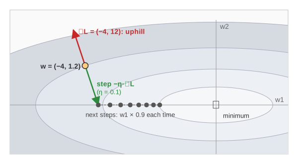
The page uses two parameters so the loss can be drawn as a map: darker cells are higher loss, ★ is the minimum. Each dot is one step. The chart under the map shows how far the loss is above its minimum (L − L*), on a log scale.
The gradient points uphill
For L = ½(w1² + 10·w2²) the gradient is ∇L = (∂L/∂w1, ∂L/∂w2) = (w1, 10·w2). At w = (−4, 1.2) that is (−4, 12): the loss rises much faster along w2 than along w1. The red arrow on the map is this direction. Its length (‖∇L‖) says how steep the slope is.
The update rule
w ← w − η·∇L(w). The learning rate η scales the step (the green arrow). Near a minimum the gradient gets small, so the steps get small by themselves: on the round bowl with η = 0.1 every step multiplies w by exactly 0.9. (Demo 1: round bowl)
Choosing the learning rate
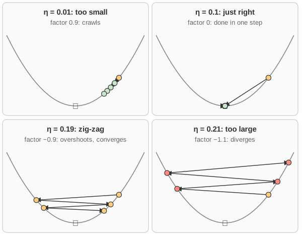
Along a direction where the loss curves with strength λ (an eigenvalue of the Hessian; 1 and 10 for the valley), one step multiplies the distance to the minimum by 1 − η·λ.
| η on the valley (λ = 1 and 10) | factor along w1 | factor along w2 | what you see |
|---|---|---|---|
| 0.01 | 0.99 | 0.9 | too small: crawls, after 50 steps still far away |
| 0.1 | 0.9 | 0 | good: w2 is solved in one step, w1 shrinks by 0.9 |
| 0.19 | 0.81 | −0.9 | zig-zag across the valley, but converges |
| 0.21 | 0.79 | −1.1 | diverges: each step overshoots more than the last |
So η must stay below 2/λmax. (Demo 2, Demo 3)
Ill-conditioning and momentum
When one direction is much steeper than another (the valley's condition number is 10), the steep direction forces a small η and the flat direction then moves slowly. Momentum keeps a velocity: v ← β·v + ∇L, w ← w − η·v, with β = 0.9. Gradient components that keep their sign (along the valley floor) add up; components that flip sign (across the valley) cancel. On the valley with η = 0.02, plain gradient descent is still not converged after 160 steps, while momentum gets there in about 150. (Demo 4)
Batch, mini-batch and SGD
A real loss is an average over training samples: here the mean squared error of a line ŷ = a·x + b over 8 points. Its gradient is an average too. Full batch uses all 8 samples per step; mini-batch uses 2; stochastic gradient descent (SGD) uses 1. Fewer samples give a cheaper but noisy estimate of the same gradient. In one epoch (one pass over the data) full batch takes 1 step, mini-batch 4, SGD 8 — so for the same work SGD gets further, along a jagged path. (Demo 6)
Local minima and saddle points
If the loss is not convex, gradient descent finds a minimum, not the minimum: it rolls into the basin it starts in. On the two-minima surface a start at (1.5, 1) ends in the local minimum near w1 = 0.96, a start at (−0.5, 1) ends in the global one near w1 = −1.04. (Demo 5) In high dimensions true local minima are rarer than saddle points and flat plateaus, where the gradient is small and progress stalls.
Beyond momentum
Adam and RMSProp scale each parameter's step by a running average of its squared gradient, so steep and flat directions get similar step sizes. Learning-rate schedules (warm-up, decay) use a large η early and a small one near the end.
Where does the gradient come from?
For a neural network with millions of weights, the gradient is computed by backpropagation: the chain rule applied from the loss backwards through the network. See Backpropagation.
What the page leaves out
Real models have millions of parameters, so the loss cannot be drawn; the two-parameter map is only an analogy. Nesterov momentum, Adam, weight decay, gradient clipping and learning-rate schedules are only described, not animated. The divergence test is simply "the point left the map".