The problem: finding one row without reading the table
A table's rows have to live somewhere on disk. The simplest arrangement, and the one almost every database uses by default, is a heap file: a sequence of fixed-size pages (commonly 4KB, 8KB or 16KB), each holding as many rows as fit. A new row goes into whichever page has room. There is no order to it — the heap file is a pile, not a sorted list.
That makes writing cheap and reading expensive. SELECT * FROM people WHERE id = 42 has no idea which page holds id 42, so the database has to read every page and look at every row: a full table scan, costing one page read per page in the table. For a million-row table that is tens of thousands of disk reads to return a single row.
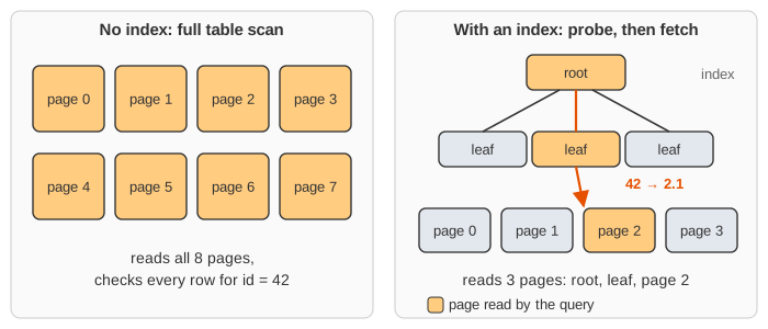
An index is a second structure, kept alongside the table, whose only job is to answer the question which page and slot holds the row with this key? On this page the visualization shows both halves at once: the index on top, the heap file below.
The index here is a B+ tree. If you want the structure on its own first — splits and merges, insertion and deletion, with no database around it — the B+ tree visualization is the place to start; this page picks it up from there and puts it to work.
Row addresses: the RID
Every row has an address, called the RID (row id) or tuple id: the pair (page number, slot number). In the visualization a RID is written 2.1 — page 2, slot 1 — and each slot in the heap file is labelled with its own address so you can follow them.
A RID is not a memory pointer. It is a position in a file, so it stays valid after the database restarts, and it is small — a few bytes — which is why an index can hold many of them in one page.
Why a B+ tree, and not a binary search tree
A balanced binary search tree finds a key in O(log2 n) comparisons, which sounds like enough. But a database does not pay for comparisons, it pays for page reads, and each node of a binary tree sits somewhere different on disk. A million rows means about 20 nodes on the search path, and therefore about 20 page reads — where each read is thousands of times slower than a comparison in memory.
The B+ tree fixes this by making every node exactly one page. A node then holds not two children but as many as fit. With 4KB pages, 4-byte keys and 6-byte pointers, a node holds roughly 400 children — its fanout. The height of the tree is log400 n rather than log2 n:
| 1 level (root only) | up to ~400 entries | 1 page read |
| 2 levels | up to ~160 000 entries | 2 page reads |
| 3 levels | up to ~64 000 000 entries | 3 page reads |
| 4 levels | up to ~25 000 000 000 entries | 4 page reads |
Three page reads into a 64-million-row table is the whole reason indexes exist. And because the root, and usually the entire second level, stay cached in memory, a lookup often costs just one real disk read — the leaf — plus one for the row itself.
The visualization uses a max degree of 3 to 5 instead of 400, because 400 keys per node will not fit on a screen. Everything else is the same; only the numbers shrink.
What is in a node
- Internal nodes hold only separator keys and child pointers. A separator is a signpost, not data: the key 30 in an internal node means everything below the pointer to my left is under 30, everything below the pointer to my right is 30 or more. The row with id 30 is not stored there.
- Leaf nodes hold the entries: a key together with the RID of the row that has that key, drawn
30→2.1. Every key in the table appears in exactly one leaf, and all the leaves are at the same depth. - The leaves are chained left to right by a pointer from each leaf to the next. This is the one structural difference from a plain B tree, and it is what makes range queries cheap.
Keeping the data out of the internal nodes is what gives the B+ tree its fanout: a separator is just a key and a pointer, so more of them fit in a page, so the tree is shallower.
Inserting a row
Press Insert Row and watch the two halves happen in order:
- Store the row. The database looks for a heap page with a free slot and writes the row there. Only now does the row have an address.
- Tell the index. Walk down from the root comparing the new key with the separators until you reach the leaf where it belongs, and insert the entry
key→RIDthere, in key order. - Split if the leaf overflowed. A node that ends up with more than d−1 keys is split in two and a key is passed up to the parent — which may split in turn, all the way to the root. When the root splits, the tree gains a level; that is the only way a B+ tree ever gets taller, which is why all the leaves stay at the same depth.
Leaf splits and internal splits differ in one important detail. When a leaf splits, the key that goes up to the parent is copied: the entry has to stay in the leaf, because the leaves hold all the data. When an internal node splits, the middle key moves up and is gone from both halves — it was only a signpost, and the parent is a better place for it.
This is also where the cost of an index shows up. Every INSERT into the table now has to write the heap page and at least one index page, and a split writes several. A table with five indexes pays that five times over on every insert, update of an indexed column, and delete. Indexes are a trade: reads get cheaper, writes get more expensive, and the storage is not free either.
A point query: index probe, then heap fetch
SELECT * FROM people WHERE id = 42 with Find Row:
- Read the root. Compare 42 with its separators to pick a child.
- Repeat down the tree, one page read per level, until you reach a leaf.
- Scan the leaf for the key 42. If it is not there, the row does not exist — and notice the table itself was never touched.
- The entry gives the RID
2.1. Read heap page 2 — a database always reads a whole page, never a single row — and take slot 1. That is the row.
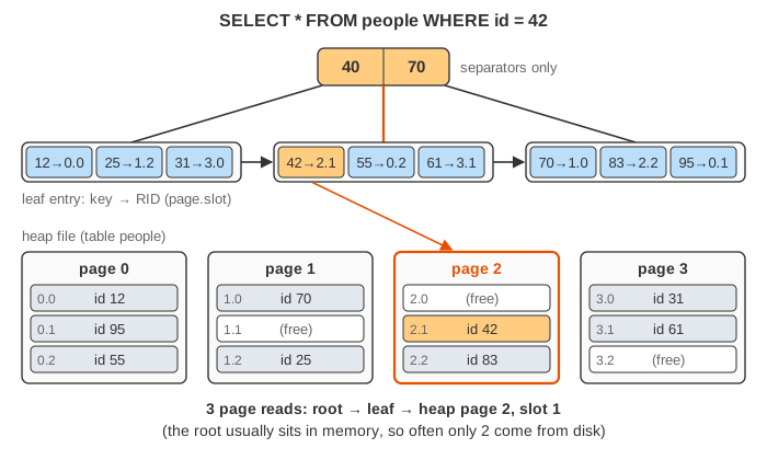
The last step is the heap fetch (or "bookmark lookup"), and it is a separate cost from walking the index. It matters enough that databases avoid it when they can: if a query only needs columns that are already in the index — SELECT id FROM people WHERE id = 42 — the index alone answers it and the heap fetch is skipped. That is called a covering index, and the plan is an index-only scan.
A range query: the leaf chain
SELECT * FROM people WHERE id BETWEEN 30 AND 70 with Range Find:
- Walk down the tree once, looking for the low end of the range, 30.
- Read the matching entries left to right in that leaf, fetching each row by its RID.
- At the end of the leaf, follow the chain pointer to the next leaf. No walking back up the tree — that is exactly what the chain is for.
- Stop at the first key above 70. Everything to the right is larger, so the rest of the table is never read.
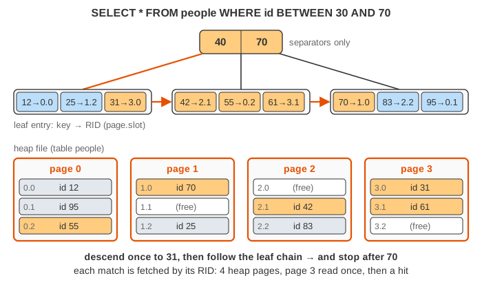
Watch the page reads while it runs. The first row on a heap page costs a read; a second row on the same page costs nothing, because the page is already in memory — that is the buffer pool, the cache of recently used pages every database keeps. It is also why the visualization's counter can stop rising partway through a scan.
But notice what the counter does on a wide range: chasing one RID per row into scattered pages can easily cost more reads than simply reading the table from front to back. The index is not free just because it exists. A query planner estimates how many rows a condition will match and picks a scan when the answer is "most of them" — which is why adding an index sometimes changes nothing at all.
This is the capability a hash index does not have. A hash index answers id = 42 in about one page read, faster than a B+ tree — but it scatters neighbouring keys to unrelated buckets on purpose, so BETWEEN 30 AND 70, id > 30, ORDER BY id and MIN(id) are all impossible without reading everything. That is why the B+ tree, not the hash table, is the default index in essentially every relational database.
A worked example
The page opens with a random table of 24 people spread over 8 heap pages, with the index already built over it, so there is nothing to type: press Find Row with the box empty and it picks an id that is really there, or Range Find with both boxes empty for a range a few rows wide. Fill a box in when you want a particular value — an id that is not in the table shows the miss instead. Insert Row with an empty box makes up an unused id, and Random Table starts over with a fresh 24 rows.
At the default max degree of 4 the index comes out three levels deep, so a point query reads 3 index pages and 1 heap page: total 4, against 8 for a full table scan. The index wins, but only by half — and that is with a table of 24 rows. The ratio is what to watch, not the numbers: every time the table grows by a factor of the fanout, the scan gets that much more expensive while the index costs one more read. Drop the max degree to 3 and watch the tree go to four levels and the cost climb, which is exactly what a small fanout does to a real index.
Now try a wide range, or press Range Find a few times. Some ranges cost less than the scan, some cost more — chasing one RID per row into scattered pages adds up fast. That crossover is real, and it is the whole job of a query planner: estimate how many rows the condition matches, then decide whether to use the index at all.
That is worth sitting with, because it is true of real databases too. An index is not automatically faster. Its advantage grows with the size of the table and shrinks with the fraction of rows the query returns. Scale the same structure to a million rows in 20 000 pages and the point query still costs 3 or 4 reads while the scan costs 20 000 — but a query that matches half the table is faster with a scan, because following 500 000 RIDs into scattered pages is worse than reading every page once in order. Query planners choose between the two for exactly this reason, using statistics about how selective the condition is.
Common mistakes, edge cases and variants
- Expecting an index to be used when the column is wrapped in a function. An index on
idorders rows byid, not byid % 10orUPPER(name).WHERE UPPER(name) = 'EVE'cannot use an index onname— you need an index on the expression itself. - A leading wildcard.
LIKE 'Ev%'is a range over keys starting with "Ev" and the index handles it.LIKE '%ve'is not a range at all, and no B+ tree can help. - Indexing a low-selectivity column. An index on a column with two distinct values sends the planner chasing RIDs for half the table; a scan is cheaper, so the index is ignored and only slows down writes.
- Assuming the index holds the rows. In a secondary index it holds only addresses, which is why the heap fetch exists. In a clustered index (a primary key in MySQL's InnoDB, for instance) the leaves hold the whole row, so there is no second read — but then the secondary indexes have to store the primary key instead of a RID, and a lookup through one costs a walk down two trees.
- Composite index column order. An index on
(city, id)sorts by city first, so it answersWHERE city = 'Hue' AND id > 40andWHERE city = 'Hue', but notWHERE id > 40alone. The usable prefix is always leftmost-first. - Deletes and free space. Removing a row leaves a hole in a heap page that a later insert can reuse, and removing an index entry may leave a leaf below half full, so the tree borrows from a sibling or merges two nodes — the mirror image of a split. Deletion is not shown on this page; the B+ tree page animates it on the bare structure.
Where this is used
Every mainstream relational database indexes with a B+ tree by default: PostgreSQL (btree, over a heap file with tuple ids exactly as drawn here), MySQL's InnoDB (a clustered B+ tree on the primary key, plus secondary B+ trees), SQLite, Oracle, SQL Server and DB2. The same structure holds up file systems (NTFS, ext4, XFS, APFS, Btrfs) and key-value stores such as LMDB and Berkeley DB. It was published by Rudolf Bayer and Edward McCreight in 1972 and has not been displaced in half a century — its only serious rival for write-heavy workloads is the LSM tree used by RocksDB and Cassandra. See also LSM tree vs B+ tree, which runs both on the same writes and reads.