B⁺ Trees Visualization

1. What is a B+-tree?

Most queries can be executed more quickly if the values are stored in order. But it's not practical to hope to store all the rows in the table one after another, in sorted order, because this requires rewriting the entire table with each insertion or deletion of a row.

This leads us to instead imagine storing our rows in a tree structure. Our first instinct would be a balanced binary search tree like a red-black tree, but this really doesn't make much sense for a database since it is stored on disk. You see, disks work by reading and writing whole blocks of data at once — typically 512 bytes or four kilobytes. A node of a binary search tree uses a small fraction of that, so it makes sense to look for a structure that fits more neatly into a disk block.

Hence the B+-tree, in which each node stores up to d references to children and up to d − 1 keys. Each reference is considered “between” two of the node's keys; it references the root of a subtree for which all values are between these two keys.

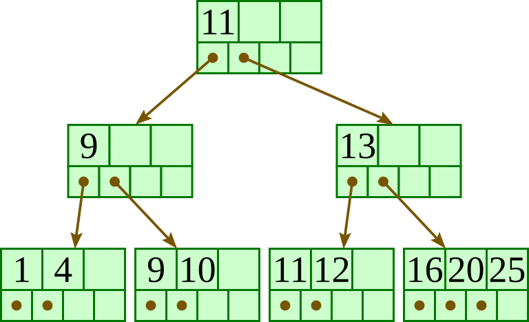
Here is a fairly small tree using 4 as our value for d.

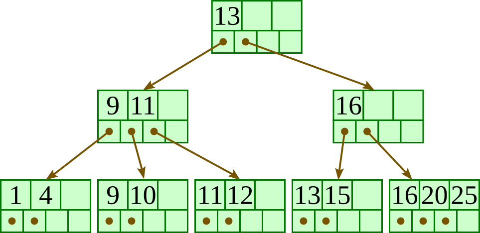
A B+-tree requires that each leaf be the same distance from the root, as in this picture, where searching for any of the 11 values (all listed on the bottom level) will involve loading three nodes from the disk (the root block, a second-level block, and a leaf).

In practice, d will be larger — as large, in fact, as it takes to fill a disk block. Suppose a block is 4KB, our keys are 4-byte integers, and each reference is a 6-byte file offset. Then we'd choose d to be the largest value so that 4 (d − 1) + 6 d ≤ 4096; solving this inequality for d, we end up with d ≤ 410, so we'd use 410 for d. As you can see, d can be large.

A B+-tree maintains the following invariants:

• Every node has one more references than it has keys.
• All leaves are at the same distance from the root.
• For every non-leaf node N with k being the number of keys in N: all keys in the first child's subtree are less than N's first key; and all keys in the ith child's subtree (2 ≤ i ≤ k) are between the (i − 1)th key of n and the ith key of n.
• The root has at least two children.
• Every non-leaf, non-root node has at least floor(d / 2) children.
• Each leaf contains at least floor(d / 2) keys.
• Every key from the table appears in a leaf, in left-to-right sorted order.

In our examples, we'll continue to use 4 for d. Looking at our invariants, this requires that each leaf have at least two keys, and each internal node to have at least two children (and thus at least one key).

2. Insertion algorithm

Descend to the leaf where the key fits.

1. If the node has an empty space, insert the key/reference pair into the node.
2. If the node is already full, split it into two nodes, distributing the keys evenly between the two nodes. If the node is a leaf, take a copy of the minimum value in the second of these two nodes and repeat this insertion algorithm to insert it into the parent node. If the node is a non-leaf, exclude the middle value during the split and repeat this insertion algorithm to insert this excluded value into the parent node.

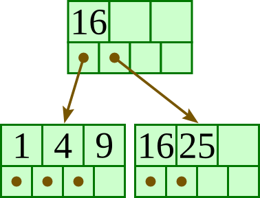
Initial:

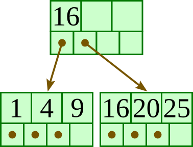
Insert 20:

Insert 13:

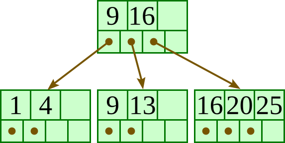
Insert 15:

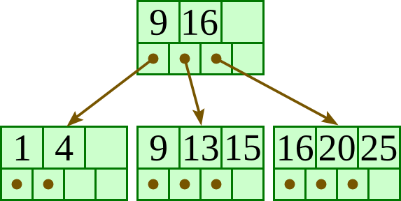
Insert 10:

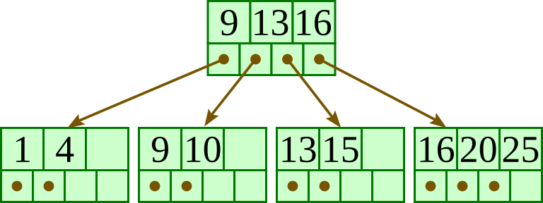
Insert 11:

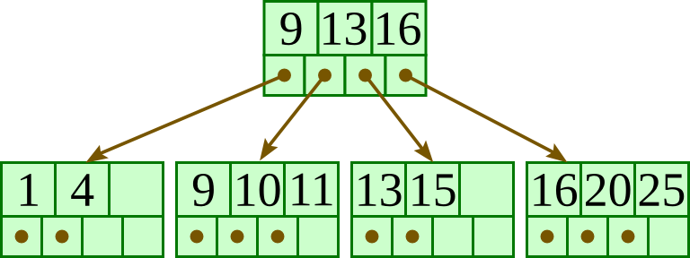
Insert 12:

3. Deletion algorithm

Descend to the leaf where the key exists.

1. Remove the required key and associated reference from the node.
2. If the node still has enough keys and references to satisfy the invariants, stop.
3. If the node has too few keys to satisfy the invariants, but its next oldest or next youngest sibling at the same level has more than necessary, distribute the keys between this node and the neighbor. Repair the keys in the level above to represent that these nodes now have a different “split point” between them; this involves simply changing a key in the levels above, without deletion or insertion.
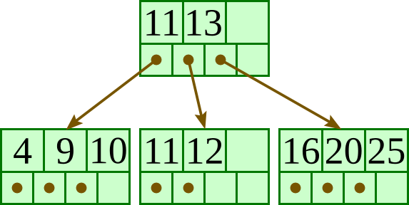
4. If the node has too few keys to satisfy the invariant, and the next oldest or next youngest sibling is at the minimum for the invariant, then merge the node with its sibling; if the node is a non-leaf, we will need to incorporate the “split key” from the parent into our merging. In either case, we will need to repeat the removal algorithm on the parent node to remove the “split key” that previously separated these merged nodes — unless the parent is the root and we are removing the final key from the root, in which case the merged node becomes the new root (and the tree has become one level shorter than before).

Initial:

Delete 13:

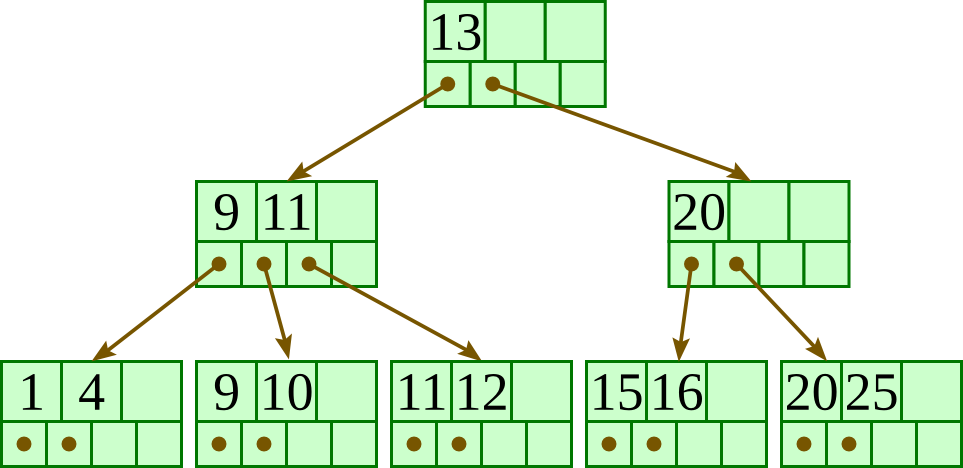
Delete 15:

Delete 1:

4. Seeing it work as a database index

This page shows the B+-tree on its own: keys going in and coming out, nodes splitting and merging. But the structure was invented for a job, and the job is finding rows in a table.

The B+ tree as a database index visualization shows that job being done. The same tree sits on top, but its leaves hold index entries — a key paired with the address of a row — and underneath it is the heap file where the rows themselves live, a handful of fixed-size pages with a few rows each. A row's address, its RID, is simply the pair (page number, slot number).

With both halves on screen you can follow what a database actually does:

• An insert happens in two steps, and in this order: the row is written into a heap page, which is what gives it an address, and only then is the entry key → address added to the leaf where it belongs (splitting upward, exactly as on this page).
• A lookup walks from the root to a leaf, one page read per level, finds the entry, and then follows the address into the heap file to fetch the row. The index knows where the row is; it does not hold the row.
• A range query walks down once and then runs along the chain of leaf pointers, which is the one thing this page draws that a plain B-tree has not got, and the reason a B+-tree beats a hash index for anything but single-key lookups.

Every step there is counted in page reads, against what it would cost to read the whole table instead — which is the only measure a database really cares about.

This is not a niche structure. Every mainstream relational database indexes with a B+-tree: PostgreSQL, MySQL's InnoDB, SQLite, Oracle, SQL Server and DB2. So do the key-value stores LMDB and Berkeley DB, and the filesystems NTFS, APFS, XFS and Btrfs, which face the same problem of finding a record on a disk that is read a block at a time. Bayer and McCreight published the idea in 1972, and half a century later nothing has displaced it for on-disk indexing; its only serious rival, the LSM tree used by RocksDB and Cassandra, trades read speed for write speed rather than beating it outright.