Fibonacci heaps: be lazy now, tidy up later
A Fibonacci heap (Michael Fredman and Robert Tarjan, 1984) is a mergeable priority queue designed to make insert, merge and above all decreaseKey cost O(1) amortized time, while removeSmallest (extract-min) stays O(log n) amortized. That combination is what graph algorithms such as Dijkstra's and Prim's need: they call decrease-key up to once per edge but extract-min only once per vertex.
A binary heap cannot do this: every insert and decrease-key moves an item up a path of length up to lg n, and merging two array heaps costs Θ(n). A binomial queue merges in O(log n) but still does work on every insert. The Fibonacci heap's idea is laziness: insert and merge just add trees to a list and do no restructuring at all. The clean-up, called consolidation, happens only in extract-min, when the heap has to search for the new minimum anyway.
The structure
- A collection of heap-ordered trees (every key ≤ its children's keys). There is no limit on how many trees there are, or on two trees having the same degree.
- The roots are kept in a doubly linked root list (circular in most textbooks), and a pointer min points at the smallest root.
- Each node stores its key, its degree (number of children), a parent pointer, a pointer to one child, left and right sibling pointers, and a boolean mark. A node is marked when it has lost a child since it last became a child of another node.
The operations
insert(x):         make x a one-node tree, add it to the root list
                   if x.key < min.key: min = x                 // O(1)

merge(H1, H2):     concatenate the two root lists
                   min = the smaller of the two minimums       // O(1)

extractMin():      z = min
                   add every child of z to the root list (clear parent)
                   remove z from the root list
                   consolidate()
                   return z

consolidate():
    A[0..D] = all empty          // D = maximum possible degree
    for each tree w in the root list:
        x = w;  d = x.degree
        while A[d] is not empty:
            y = A[d]             // another tree with the same degree
            if y.key < x.key: swap x and y
            link(y, x)           // y becomes a child of x, y.mark = false
            A[d] = empty
            d = d + 1
        A[d] = x
    rebuild the root list from the trees in A, and set min to the smallest root

decreaseKey(x, k):             // requires k ≤ x.key
    x.key = k
    p = x.parent
    if p is not null and x.key < p.key:     // heap order broken
        cut(x, p)
        cascadingCut(p)
    if x.key < min.key: min = x

cut(x, p):         remove x from p's children, p.degree = p.degree - 1
                   add x to the root list, x.mark = false

cascadingCut(y):
    z = y.parent
    if z is not null:
        if y.mark is false: y.mark = true        // first child lost: remember it
        else: cut(y, z); cascadingCut(z)         // second child lost: cut y too

delete(x):         decreaseKey(x, -infinity);  extractMin()
Consolidation is the same "link two trees of equal degree" step as in a binomial queue, repeated until all roots have different degrees. The array A remembers, for each degree, the one tree of that degree seen so far.
What the animation shows
This page animates Insert, Remove Smallest and Clear Heap (tick Random for random keys); decrease-key, delete and the marks are not animated, so the trees you see here are always binomial trees. The label Min element points at the minimum root. A new key is put into the root list just to the left of the current minimum. During Remove Smallest, the removed key moves to the corner, its children are spliced into the root list where it was, and the degree array A appears at the top right as a row of boxes numbered 0 to ⌊logφ n⌋ + 1, where n is the number of keys left (one spare box above the largest possible degree). The pointer NextElem walks along the root list, and each tree is either linked with the tree in its degree's box or placed into the empty box. (If the minimum was the only root, the page just promotes its children without consolidating.) Logical Representation draws the trees; Internal Representation draws the stored pointers: double arrows between neighbouring roots and siblings, arrows between a parent and its first child, and each node's degree in blue. Keys are stored as four-digit strings, so 5 is drawn as 0005.
Worked example
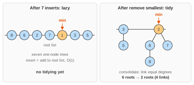
Insert 5, 3, 8, 1, 6, 2, 7, then press Remove Smallest twice. This is the order the page uses.
insert 5, 3, 8, 1, 6, 2, 7   (each new key goes just left of the minimum)
    root list:  8  6  2  7  1  3  5          min -> 1
    seven one-node trees, no work done yet

remove smallest   remove 1 (no children); consolidate 8 6 2 7 3 5:
    8: A[0] = 8
    6: A[0] holds 8, link: 6 < 8, so 6-8 has degree 1.  A[1] = 6-8
    2: A[0] = 2
    7: A[0] holds 2, link: 2-7 (degree 1)
         A[1] holds 6-8, link: 2 < 6, 2 gets child 6 (degree 2).  A[2] = 2
    3: A[0] = 3
    5: A[0] holds 3, link: 3-5 (degree 1).  A[1] = 3-5
    root list from A:
        3        2          min -> 2
        |       / \
        5      6   7
               |
               8

remove smallest   remove 2; its children 6-8 and 7 join the root list:
    list 3-5  6-8  7
    3-5: A[1] = 3-5
    6-8: A[1] holds 3-5, link: 3 < 6, 3 gets child 6 (degree 2).  A[2] = 3
    7:   A[0] = 7
    root list from A:
        7      3            min -> 3
              / \
             6   5
             |
             8
The first extract-min pays for the six cheap inserts: it does 4 links. Afterwards there are only 2 roots, one per 1-bit of 6 = 1102.
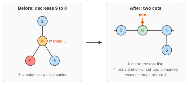
Decrease-key on paper (not animated here). Suppose node 4 was already marked because it lost a child earlier. Decreasing 9 to 0 cuts 9; its parent 4 is marked, so 4 is cut as well and unmarked; 4's parent 1 is a root, so the cascade stops:
      1                 1     0     4
      |         ->                  |
      4*                            6
     / \              min -> 0
    9   6
Why it works: the degree bound and the potential
Degree bound. Let x be any node of degree k, and list its children y1, …, yk in the order they were linked to it. When yi was linked, x already had at least i − 1 children, and links only join equal degrees, so yi had degree at least i − 1. Since then it has lost at most one child (a second loss would have cut it away), so its degree is still at least i − 2. If sk is the fewest nodes a degree-k subtree can have, this gives sk ≥ 2 + s0 + s1 + … + sk−2, and that sum is the Fibonacci recurrence: sk ≥ Fk+2 ≥ φk, where φ = (1 + √5)/2 ≈ 1.618. Hence every degree is at most D(n) = logφ n ≈ 1.44 lg n. This is where the name comes from, and it is the whole reason for the marks: cutting a node after its second lost child keeps trees "bushy enough".
Potential. Let Φ = t + 2m, with t the number of roots and m the number of marked nodes. Then:
- insert costs O(1) and raises Φ by 1: amortized O(1).
- extractMin really costs O(D + t) (each link removes a root), but afterwards at most D + 1 roots remain, so Φ falls by about t − D: amortized O(D) = O(log n).
- decreaseKey with c cuts really costs O(c); it adds c roots, unmarks at least c − 1 nodes and marks at most one, so Φ changes by at most c + 2(2 − c) = 4 − c: amortized O(1).
Running time
operation     Fibonacci heap        binomial queue   binary heap
insert        O(1)                  O(1) amortized   O(log n)
findMin       O(1)                  O(log n)         O(1)
merge         O(1)                  O(log n)         Theta(n)
extractMin    O(log n) amortized    O(log n)         O(log n)
decreaseKey   O(1) amortized        O(log n)         O(log n)
delete        O(log n) amortized    O(log n)         O(log n)
The bounds are amortized: a single extract-min after n inserts must look at all n roots and takes Θ(n) time, and a cascading cut can climb a long path. With a Fibonacci heap, Dijkstra's and Prim's algorithms run in O(E + V log V) instead of O(E log V) with a binary heap.
Common mistakes and edge cases
- Forgetting to clear marks. A node that is cut to the root list, or linked under another root, becomes unmarked.
- A too-small degree array.
Aneeds D(n) + 1 ≈ 1.44 lg n + 1 slots. This page sizes it from the number of keys on every Remove Smallest (boxes 0 to ⌊logφ n⌋ + 1), so any number of keys works; a fixed-size array silently loses every tree whose degree does not fit. - Cutting the parent too early. A parent is cut only on its second lost child; cutting on the first loss is correct but wastes work, never cutting breaks the degree bound.
- decreaseKey needs a handle (a pointer to the node). A heap cannot find a key by value quickly, so Dijkstra's algorithm keeps each vertex's node pointer.
- Constant factors. Many pointers per node and poor cache behaviour make Fibonacci heaps slower than binary or pairing heaps on typical inputs, despite the better bounds.
Variants
- Pairing heaps: much simpler, very fast in practice; decrease-key is sub-logarithmic amortized but provably not O(1).
- Rank-pairing heaps (Haeupler, Sen and Tarjan) reach the Fibonacci bounds with a simpler structure; strict Fibonacci heaps and Brodal queues achieve them in the worst case.
- Binomial queues are the eager version: link on every insert, no cuts.
Where Fibonacci heaps are used
Their main use is in the analysis and implementation of graph algorithms with many decrease-key operations: Dijkstra's shortest paths and Prim's minimum spanning tree in O(E + V log V), and faster algorithms for minimum spanning trees, weighted matching and network flow built on them. They are the standard textbook example of amortized analysis with a potential function. In practice, libraries often choose a binary, d-ary or pairing heap unless graphs are dense enough for the O(1) decrease-key to pay off.