Skew heaps: the simplest fast-merging heap
A priority queue supports insert and removeSmallest; a mergeable priority queue also supports merge (meld), which combines two queues into one. A binary heap is bad at merging: it is an array holding a complete binary tree, so two heaps cannot be linked together, and merging heaps of sizes n and m means rebuilding one big array in Θ(n + m) time.
A skew heap (Daniel Sleator and Robert Tarjan, 1986) is a heap-ordered binary tree built from pointers, with no balance rule and no extra field in the nodes at all. It is the self-adjusting version of the leftist heap: a leftist heap stores a null path length in every node and swaps a node's children only when the right side becomes "longer"; a skew heap simply swaps the children of every node on the merge path. Any single operation can be slow, but the swapping keeps the right paths short on average, and every operation costs O(log n) amortized.
The only rule: heap order
Every node's key is ≤ the keys of its children, so the minimum is at the root. There is no rule about the tree's shape; it can be very lopsided. The right path (from the root, always going right) is where merging happens.
Merge, the core operation
Keep the smaller root, merge its right subtree with the other heap, and then swap its two children:
merge(a, b):
    if a is null: return b
    if b is null: return a
    if b.key < a.key: swap a and b        // a now has the smaller root
    a.right = merge(a.right, b)            // walk down a's right path
    swap a.left and a.right                // always, no test
    return a

insert(x):         root = merge(root, new node x)
removeSmallest():  min = root.key
                   root = merge(root.left, root.right)
                   return min
The merged subtree, which just grew, moves to the left, and the old left subtree becomes the new right path. That is the "skew": the long side is pushed away from the path the next merge will follow. On this page the swap is done at every node where the recursion compared two roots; when one side is empty, the other heap is returned unchanged, without a swap.
What the animation shows
The page offers Insert, Remove Smallest and Clear Heap (tick Random to have a random key filled in). Both operations are shown as merges: a new key starts as a one-node heap at the top left, and Remove Smallest takes the root off and merges its two subtrees. The two highlight circles mark the roots being compared at each level of recursion. The winner and its left subtree are faded while its right subtree is merged, then the tree is reconnected and the message "Swapping subtrees after merge" appears as its children change sides. Keys are stored as four-digit strings, so 5 is drawn as 0005. Ties are won by the heap that was on the left.
Worked example
Insert 5, 3, 8, 1, 6, 2, then press Remove Smallest twice. These are the trees the page draws after each step.
insert 5    5

insert 3    3 < 5, 3.right = merge(null, 5) = 5, then swap:
               3
              /
             5

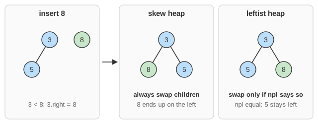
insert 8    3 < 8, 3.right = merge(null, 8) = 8, then swap.
            (A leftist heap would keep 5 on the left; a skew heap swaps anyway.)
               3
              / \
             8   5

insert 1    1 < 3, 1.right = the 3-heap, then swap:
                 1
                /
               3
              / \
             8   5

insert 6    1 < 6, 1.right = merge(null, 6) = 6, then swap:
                 1
                / \
               6   3
                  / \
                 8   5

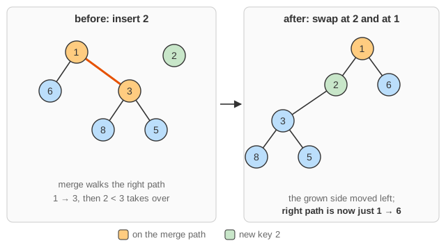
insert 2    1 < 2: 1.right = merge(3-heap, 2)
              2 < 3: 2.right = merge(null, 3-heap) = 3-heap, swap at 2
            swap at 1:
                   1
                  / \
                 2   6
                /
               3
              / \
             8   5

remove      Take 1 away, merge(2-heap, 6):
smallest    2 < 6, 2.right = merge(null, 6) = 6, swap at 2:
                 2
                / \
               6   3
                  / \
                 8   5

remove      Take 2 away, merge(6, 3-heap):
smallest    3 < 6: 3.right = merge(5, 6)
              5 < 6: 5.right = merge(null, 6) = 6, swap at 5
            swap at 3:
                 3
                / \
               5   8
              /
             6
Compare the same keys on the leftist heap page: the trees differ because the skew heap never looks at path lengths, but both stay heap-ordered and both keep the right path short.
Why it is fast on average: the amortized analysis
Call a node heavy if its right subtree has more nodes than its left subtree, and light otherwise. Use the number of heavy nodes as a potential function Φ (a "bank account" of saved-up work).
- On any right path, there are at most lg n light nodes: stepping right from a light node at least halves the number of nodes below you.
- The cost of a merge is the number of nodes on the two right paths it walks. Suppose h of them are heavy and l are light, with l ≤ 2 lg n.
- Every node on the merge path has its children swapped. A heavy node's old right subtree was the big one, and it only grows before moving to the left, so every heavy node on the path becomes light: Φ drops by h. At most the l light nodes can become heavy.
- Amortized cost = actual cost + change in Φ ≤ (h + l) + (l − h) = 2l ≤ 4 lg n, which is O(log n).
Since Φ starts at 0 and is never negative, any sequence of m operations on heaps of at most n nodes costs O(m log n) in total, even though one particular operation may walk a right path of length Θ(n).
Running time
operation        skew heap (amortized)   one operation (worst)   binary heap
findMin          O(1)                    O(1)                    O(1)
insert           O(log n)                O(n)                    O(log n)
removeSmallest   O(log n)                O(n)                    O(log n)
merge            O(log n)                O(n)                    Theta(n)
Compared with a leftist heap, a skew heap has the same bounds, but amortized instead of worst case. In exchange there is no npl field to store or update, and the code is shorter.
Common mistakes and edge cases
- Swapping conditionally. Testing sizes or path lengths before swapping turns it into a (possibly broken) leftist heap. The skew heap swaps every time.
- Deep recursion. Because a single right path can be Θ(n) long, a recursive merge can overflow the call stack on big inputs. Production code uses an iterative, top-down merge: splice the two right paths together in sorted order, then swap children along the result.
- Amortized does not mean every operation is fast. Do not use skew heaps where each single operation must meet a deadline.
- Books differ on whether the last node of the merge path (where one side becomes empty) also has its children swapped. Both versions have the same amortized bound.
- Removing from an empty heap does nothing on this page; a real implementation should report an error.
Variants
- Leftist heaps keep null path lengths and swap only when needed, for worst-case O(log n).
- Pairing heaps are another self-adjusting heap, with O(1) insert and merge and fast decrease-key in practice.
- Skew binomial heaps are a different structure (a binomial-queue variant) despite the similar name.
Where skew heaps are used
Skew heaps are popular whenever a small, correct, mergeable priority queue is needed: in functional programming, where merge-based heaps are natural; in Tarjan's efficient version of Edmonds' algorithm for minimum spanning arborescences (directed MST), where the queues of incoming edges of contracted vertices are merged; in scheduling and discrete-event simulation; and in programming contests, where "merge two priority queues" appears as a sub-problem and the whole structure fits in a dozen lines.