The idea: keep one Gaussian and fix it with each reading
A cart drives along a track. It is told to move +2 m each step, but bumps push it a little off. A sensor reads its position every step, with noise. The Kalman filter keeps its belief about the position as one Gaussian (bell curve): a best guess, the mean x̂, and how unsure it is, the variance P. Each step has two halves. Predict moves the belief like the cart. Update blends it with the new reading.
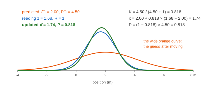
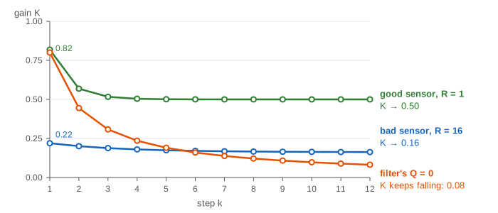
Press Predict and then Update to run one step at a time, Cycle for both, or pick a demo and press Run Demo. The top panel shows the true cart (the filter never sees it), the readings (blue dots) and the estimates (green dots). The middle panel draws the Gaussians. The bottom left shows the formulas with this step's numbers; the bottom right shows the gain K of every step.
Predict: shift and widen
The filter knows the command u = +2 m. So it moves its guess by u and adds the process noise Q, the variance of the bumps it expects:
- x̂⁻ = x̂ + u
- P⁻ = P + Q
The minus sign means "before the reading". Variances of independent errors add, so the curve always gets wider when it moves. Driving without looking can only add doubt. In Demo 1 the belief N(0, 4) becomes N(2.00, 4.50) (Demo: one cycle, step by step).
Update: the Kalman gain
The sensor reads z with measurement noise of variance R. The filter weighs the reading by the Kalman gain K:
- K = P⁻ / (P⁻ + R)
- x̂ = x̂⁻ + K (z − x̂⁻)
- P = (1 − K) P⁻
z − x̂⁻ is the innovation: how far the reading is from what the filter expected. K says how much of that gap to accept. In Demo 1, P⁻ = 4.50 and R = 1, so K = 4.50 / 5.50 = 0.818. The reading 1.68 is far more trusted than the guess 2.00, and the new mean is 1.74. P drops to 0.818, below both 4.50 and 1. This is Bayes' rule for Gaussians: the prediction is the prior, the reading is the likelihood, and their product is again a Gaussian (see the Normal Distribution for the curve itself).
| when | K | the filter |
|---|---|---|
| prediction very unsure (P⁻ ≫ R) | near 1 | jumps to the reading |
| both equally sure (P⁻ = R) | 0.5 | goes halfway |
| sensor very noisy (R ≫ P⁻) | near 0 | barely moves; keeps its prediction |
The gain shrinks, then settles
Every update makes P smaller, so the next K is smaller too. But each predict adds Q back, so P cannot reach 0. The two meet at a steady state. With Q = 0.5 and R = 1 it is P = 0.5, P⁻ = 1 and K = 0.5: the gains run 0.818, 0.569, 0.517, 0.504, 0.501 and then stay at 0.500 (Demo: track 12 steps, good sensor). Over the 12 steps the filter's mean error is 0.40 m, about half the raw sensor's 0.78 m.
A very unsure start only changes the first steps. With P₀ = 100 the first gain is 0.990, so the filter almost copies the first reading (1.68); the next gains are 0.598 and 0.523, nearly the same as before (Demo: unsure start). Note that K and P do not depend on the readings at all. They can be computed before the run.
A good sensor and a bad one
Demo 3 uses the same noise, but the sensor's variance is R = 16 m² (a standard deviation of 4 m instead of 1 m). Now K starts at 0.220 and settles at 0.163: each reading moves the estimate only a sixth of the way. One reading says 20.45 m while the cart is at 10.10 m; the estimate moves only to 12.12 m. Over 12 steps the filter's mean error is 0.64 m while the readings are off by 3.13 m on average. The price is lag: P stays at 2.61, and a real turn of the cart would show up slowly (Demo: bad sensor).
Missed readings
If a reading is lost, the filter just predicts again. P grows by Q at every step: 1.017, 1.517, 2.017, 2.517 over four steps without a reading. When a reading finally arrives, the gain is high (0.716), and the estimate jumps most of the way to it (Demo: sensor drops out).
When Q is wrong
Q is a design choice: how much the filter expects the cart to wander. If the filter assumes Q = 0, it believes the cart follows u exactly. Then P only shrinks, K falls roughly like 1/k (0.800, 0.444, 0.308, … 0.082), and later readings barely count. The real cart does wander, so the estimate falls behind: at step 12 it is 1.90 m off, worse than the raw reading (1.47 m) (Demo: filter assumes Q = 0). Too small a Q makes the filter over-confident; too large a Q makes it jumpy.
Kalman filter and particle filter
| Kalman filter | particle filter | |
|---|---|---|
| belief | one Gaussian: x̂ and P | N weighted samples |
| models | linear motion and sensor, Gaussian noise | any motion and sensor model |
| several possible places | no | yes |
| cost per step | a few multiplications | grows with N |
| result | exact when the models hold | approximate, better with more samples |
The Kalman filter is a least-squares estimate updated one reading at a time; linear regression fits all the data at once by the same squared-error idea.
On the canvas, when a curve would be too tall for the belief panel, all three curves are shrunk by the same factor, and the panel says so (for example "heights × 0.41 to fit" at the end of Demo 6). Their shapes and positions stay exact.
What the page leaves out
More than one state variable (position and velocity, with matrices F, H, Q, R and the covariance matrix), the extended and unscented Kalman filters for nonlinear models, the information form, smoothing (using later readings to fix earlier estimates), how Q and R are tuned or estimated in practice, outlier rejection by gating the innovation, and numerical tricks such as the Joseph form of the covariance update.