The idea: a bell set by two numbers
Heights, measurement errors and test scores pile up around an average and thin out on both sides in the same smooth, symmetric shape: the normal distribution, or bell curve. It is fixed by two numbers. The mean μ is the centre of the bell. The standard deviation σ is its width: the distance from μ to the point where the curve turns from bending down to bending up. We write N(μ, σ²).
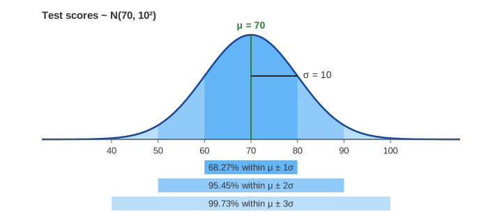
The page models test scores with μ = 70 and σ = 10. The bell on the canvas is built from thin slices so that any part of the area can be shaded. The total area under the curve is 1 (100% of the scores), and the area over a range is the fraction of scores in that range.
Changing μ and σ
The curve is f(x) = e^(−(x − μ)²/(2σ²)) / (σ√(2π)). Changing μ slides the whole
bell left or right without changing its shape. Changing σ stretches it: because the total area
must stay 1, a wider bell is also lower. Its peak is 1/(σ√(2π)), so σ = 15 gives a peak only 2/3 as tall as
σ = 10 (Demo: changing μ and σ).
The 68–95–99.7 rule
For every normal distribution, the same fraction of the area lies within a given number of standard deviations of the mean (Demo: the 68–95–99.7 rule):
| Range | Scores, μ = 70, σ = 10 | Area inside | Outside |
|---|---|---|---|
| μ ± 1σ | 60–80 | 68.27% | about 1 in 3 |
| μ ± 2σ | 50–90 | 95.45% | about 1 in 22 |
| μ ± 3σ | 40–100 | 99.73% | about 3 in 1000 |
This is the quick sanity check behind "three-sigma" limits in quality control: a value more than 3σ from the mean is rare enough to deserve a second look.
z-scores and the z table
To find the fraction below a score you would need the area under this bell. Instead of a table for every μ and σ, every score is moved onto one bell, the standard normal N(0, 1), with the z-score
z = (x − μ) / σz counts how many standard deviations x lies above (z > 0) or below (z < 0) the mean. The area left of z, written Φ(z), is listed in a z table; as a percentage it is the percentile. A score of 85 when μ = 70 and σ = 10 gives z = (85 − 70)/10 = 1.5 and Φ(1.5) = 0.9332: the student did better than 93.3% of all students, the 93rd percentile (Demo: score 85 → z = 1.5 → 93rd percentile).
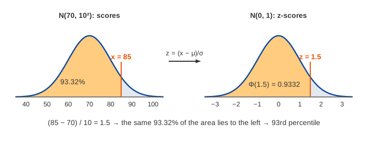
A table usually lists only z ≥ 0. For a negative z use the symmetry of the bell: Φ(−z) = 1 − Φ(z). A score of 55 gives z = −1.5 and Φ = 1 − 0.9332 = 0.0668, the 6th percentile.
| z | Φ(z) | z | Φ(z) |
|---|---|---|---|
| 0.0 | 0.5000 | 1.96 | 0.9750 |
| 0.5 | 0.6915 | 2.0 | 0.9772 |
| 1.0 | 0.8413 | 2.5 | 0.9938 |
| 1.5 | 0.9332 | 3.0 | 0.9987 |
Comparing two scores
Raw scores from different tests are not comparable, but z-scores are. Ann scores 85 on test A (μ = 70, σ = 10); Ben scores 88 on test B (μ = 80, σ = 8). Ben has more points, but his z = (88 − 80)/8 = 1.0 (84th percentile) is below Ann's z = 1.5 (93rd percentile): relative to the others who took the same test, Ann did better (Demo: compare scores from two tests).
Confidence intervals
In practice μ is unknown and we only see a sample. The page draws n = 25 scores and takes their mean x̄. By the central limit theorem x̄ is itself normal, with mean μ and standard deviation σ/√n, the standard error (10/5 = 2 points). Since 95% of a normal lies within 1.96 standard deviations, x̄ lands within 1.96·σ/√n of μ in 95% of samples, so the 95% confidence interval
x̄ ± 1.96 · σ / √n = x̄ ± 3.92 (σ = 10, n = 25)contains μ in 95% of samples. The page draws 20 seeded samples: 19 intervals cover μ = 70 and sample #12 (x̄ = 66.05) misses. Drawing 80 more brings the total to 95 of 100 (Demo: 95% confidence intervals cover μ).
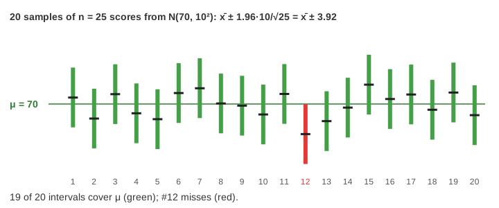
"95% confidence" does not mean a given interval has a 95% chance of holding μ: μ is a fixed number, so each interval either holds it or not. It means the recipe catches μ 95% of the time. A wider interval (99%, z = 2.58) misses less often; a bigger n makes every interval narrower, like 1/√n. The same intervals decide A/B tests: if the interval for the difference between two variants excludes 0, the difference is significant at the 5% level. Bayes' theorem gives the other view, a probability for μ itself after seeing the data.
See also Mean vs Median vs Mode: on a symmetric bell all three coincide at μ, but an outlier or a skewed tail pulls them apart.
For counts of rare events the better approximation is Poisson, not normal: Binomial vs Poisson.
See also hypothesis testing with a coin: the p-value as a tail area, α, type I/II errors and power; a 95% interval excludes a value exactly when the two-sided test rejects it at α = 0.05.
See also Confidence Intervals: hundreds of repeated samples, the effect of n and of the 80–99% level, and why exactly the samples whose x̄ falls outside μ ± E miss.
Generative diffusion models add normal noise to data step by step until it becomes N(0, I), then learn to remove it.
Each velocity component of a gas molecule is normally distributed, which gives the speeds the Maxwell–Boltzmann shape on Ideal Gas and the Maxwell–Boltzmann Distribution.
A mixture of several 2D normal distributions, fitted with EM, is a clustering method: see k-means vs Gaussian Mixture Model.
Where σ comes from: Variance and Standard Deviation computes it step by step as the side of the average squared deviation.
The area left of a score is the height of the CDF there: see PDF vs CDF.
For a skewed continuous distribution, see exponential waiting times between random arrivals.
See also Continuous Distributions for the uniform, normal, exponential, gamma and beta densities side by side.
See also Box Plots and IQR Outliers, where the z-score rule |z| > 3 is compared with box-plot fences and misses outliers in small or skewed samples.
See also the Kalman Filter, where a predicted Gaussian and a reading's Gaussian combine into a narrower one at every step.
See also The EM Algorithm, Step by Step, which fits a mixture of two normal distributions to data without labels.
What the page leaves out
- Unknown σ: with the sample standard deviation s in place of σ, the interval uses Student's t with n − 1 degrees of freedom instead of 1.96 (2.06 for n = 25).
- How Φ is computed: it has no closed form; the page uses a polynomial approximation of the error function.
- Checking normality (Q–Q plots), skewed and heavy-tailed data, and transformations such as logs.
- One-sided intervals, hypothesis tests and p-values, and intervals for proportions.
- The multivariate normal and correlated variables.