The idea: split, apply, combine
Many questions about a table have the form "for each X, compute Y": total sales per shop, mean score per class. pandas answers them with groupby, in three stages. Split: the rows are put into groups by the value of a key column. Apply: one calculation runs on each group on its own. Combine: the results are put together into one Series or DataFrame (Demo: split-apply-combine with sum).
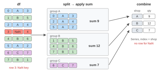
The page uses one small DataFrame df with the default index 0 to 7. Row 3 has no shop (NaN), which matters later.
| index | shop | item | qty |
|---|---|---|---|
| 0 | A | tea | 3 |
| 1 | B | milk | 5 |
| 2 | A | milk | 4 |
| 3 | NaN | tea | 4 |
| 4 | B | tea | 6 |
| 5 | A | tea | 2 |
| 6 | C | milk | 7 |
| 7 | B | milk | 1 |
df.groupby("shop") alone computes nothing. It returns a DataFrameGroupBy object that only knows which rows belong to which group (A: 0, 2, 5; B: 1, 4, 7; C: 6). The work happens when you call a method on it. Every number on the canvas is what pandas 2.3 prints for this data.
agg, transform, filter: what comes back
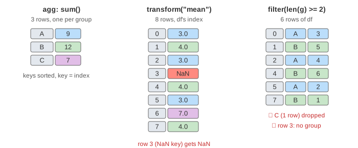
The same groups can give three different shapes of result. Which one you get depends on the method, not on the groups.
| method | apply returns, per group | combined result | on the page |
|---|---|---|---|
sum(), mean(), agg([...]) | one value (or one per function) | one row per group, indexed by the key, keys sorted | A 9, B 12, C 7 |
transform("mean") | one value per row of the group | same length and index as df | 3.0 4.0 3.0 NaN 4.0 3.0 7.0 4.0 |
filter(func) | True or False for the whole group | the original rows of the groups that passed | rows 0 1 2 4 5 7 |
An aggregation turns each group into one row. With a list, agg(["sum", "mean", "count"]) gives one column per function: A 9, 3.0, 3; B 12, 4.0, 3; C 7, 7.0, 1 (Demo: several aggregates at once). mean is a float, so it prints as 3.0. count counts non-NaN values in the column; size() counts rows.
A transform keeps the shape of df: every row gets its own group's value back, at its own index label. That is why df["qty"] - df.groupby("shop")["qty"].transform("mean") works: both sides have index 0 to 7, so pandas subtracts row by row and gets 0.0, 1.0, 1.0, NaN, 2.0, -1.0, 0.0, -3.0 (Demo: transform keeps all 8 rows). The same idea in SQL is a window function, AVG(qty) OVER (PARTITION BY shop); see SQL Window Functions.
A filter asks one yes/no question per group and keeps or drops the group's rows whole. filter(lambda g: len(g) >= 2) keeps A (3 rows) and B (3 rows) and drops C (1 row). The result is 6 rows of the original df, in their original order, not one row per group (Demo: filter keeps or drops whole groups).
The same as SQL GROUP BY
Split-apply-combine is what SQL's GROUP BY does. The canvas shows the closest SQL under each pandas line.
| pandas | SQL |
|---|---|
df.groupby("shop")["qty"].sum() | SELECT shop, SUM(qty) FROM df GROUP BY shop |
.agg(["sum", "mean", "count"]) | SUM(qty), AVG(qty), COUNT(qty) |
.transform("mean") | AVG(qty) OVER (PARTITION BY shop) |
.filter(lambda g: len(g) >= 2) | HAVING COUNT(*) >= 2, but keeping the rows: a subquery |
groupby(["shop", "item"]) | GROUP BY shop, item |
Three differences matter. pandas sorts the keys by default (sort=True); SQL gives no order without ORDER BY. The key becomes the index of the result (the grey cells on the canvas), not a normal column; as_index=False or .reset_index() turns it back into a column. And NaN keys are handled differently, below. Where GROUP BY sits in a whole query is on How a SELECT Runs.
Several keys
With a list of keys, df.groupby(["shop", "item"]), there is one group per combination that occurs in the data. Here that is 5 groups: (A, milk) 4, (A, tea) 5, (B, milk) 6, (B, tea) 6, (C, milk) 7 (Demo: two keys, five groups). (C, tea) never occurs, so it has no group and no row. The result has a MultiIndex with two levels; .unstack() would turn the item level into columns, a small pivot table. Cubes over many dimensions are on Star Schema and OLAP Cube.
NaN keys and dropna
By default groupby has dropna=True: a row whose key is NaN belongs to no group. Nothing warns you. For row 3 that means:
| method | row 3 (shop NaN), dropna=True |
|---|---|
sum() | left out: the totals add up to 28, not 32 |
transform("mean") | kept, with value NaN |
filter(...) | left out, whatever the test says |
With dropna=False, NaN is a key like any other. The sum gets a fourth row, NaN 4, sorted last (Demo: NaN key dropped, then dropna=False). SQL works the second way: GROUP BY shop always makes one group for all NULLs. So a pandas result and a SQL result over the same data can differ by exactly this row. With two keys, a NaN in any key drops the row.
apply, and why the named methods are faster
.apply(func) calls any Python function on each group and guesses from its return value whether to combine like agg, transform or filter. It is flexible but runs Python code once per group. sum, mean, count and transform("mean") with a name run in compiled code over all groups at once, so prefer them on large data. Broadcasting a group value back to every row works the same way as array broadcasting; see NumPy Broadcasting.
See also MapReduce, where the same split by key happens across many machines, and MongoDB Aggregation, whose $group stage does it on documents.
See also NumPy Views and Strides for the arrays under a DataFrame: when indexing returns a view of the same memory and when it returns a copy.
What the page leaves out
Named aggregation (agg(total=("qty", "sum"))), different functions per column, size() on the canvas, sort=False, observed for categorical keys, grouping by a function, an index level or pd.Grouper (time bins), resample, rolling and cumsum per group, pivot_table, NaN values (not keys) inside a group, and how pandas finds the groups internally (it factorizes the keys into integer codes).