Prim Minimum Cost Spanning Tree (MST) Visualization

Minimum spanning trees and Prim's algorithm

Take a connected, undirected graph whose edges have weights (think of the cost of laying a cable between two towns). A spanning tree is a set of edges that connects all n vertices without forming a cycle; it always has exactly n − 1 edges. A minimum spanning tree (MST) is a spanning tree whose total edge weight is as small as possible.

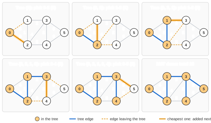
Prim's algorithm (Jarník 1930, Prim 1957, Dijkstra 1959) grows one tree from a start vertex. At every step it looks at all edges that leave the tree and adds the cheapest one, together with the new vertex at its other end. After n − 1 additions the tree spans the graph. It is a greedy algorithm: each choice looks only at the current cheapest option and is never undone.

The Known / Cost / Path table

Checking every edge that leaves the tree at every step would be slow, so the algorithm keeps one row per vertex, exactly like the table on the left of the canvas:

• Known: T once the vertex is in the tree, F otherwise (the T is greyed out, and the vertex is filled orange on the graph).
• Cost: for a vertex not yet in the tree, the weight of the cheapest edge found so far that joins it to the tree; INF if none has been seen. The start vertex has cost 0.
• Path: the tree vertex at the other end of that cheapest edge (-1 = none). At the end, every edge (Path[v], v) is an MST edge.

Each round has two phases, both animated: first all unknown Cost cells are highlighted and the smallest one is chosen; then each edge of the chosen vertex is highlighted in turn, and the page shows the comparison it makes, such as INF > 4 (update) or !(3 > 5) (no change). When the table is complete the tree edges are coloured red and the total cost is shown. You can start by typing a vertex number or by clicking a vertex.

Pseudocode

Prim(G, s):
    for each vertex v:
        known[v] = false;  cost[v] = INF;  path[v] = -1
    cost[s] = 0
    repeat n times:
        u = the unknown vertex with the smallest cost      // skip INF
        if there is none: stop                             // rest is unreachable
        known[u] = true                                    // add u (and edge path[u]-u)
        for each edge (u, v) with weight w:
            if not known[v] and w < cost[v]:
                cost[v] = w                                // cheaper link to the tree
                path[v] = u
    MST = { (path[v], v) : path[v] != -1 }

On this page, when several unknown vertices share the smallest cost, the lowest-numbered one is chosen (the scan only replaces the best on a strictly smaller cost), and an edge only replaces Path if it is strictly cheaper.

Worked example

Six vertices, start vertex 0, undirected edges (weight in brackets):

0-1 (4)   0-2 (3)   1-2 (1)   1-3 (2)   2-3 (4)
2-4 (5)   3-4 (2)   3-5 (5)   4-5 (6)

The table after each round (Known Cost Path; * marks the vertex just added):

            v=0      v=1      v=2      v=3      v=4      v=5
start      F 0  -1  F INF -1 F INF -1 F INF -1 F INF -1 F INF -1

add 0 *    T 0  -1  F 4   0  F 3   0  F INF -1 F INF -1 F INF -1
   edges 0-1: INF > 4 update;  0-2: INF > 3 update
add 2 *    T 0  -1  F 1   2  T 3   0  F 4   2  F 5   2  F INF -1
   2-0 known;  2-1: 4 > 1 update;  2-3: INF > 4;  2-4: INF > 5
add 1 *    T 0  -1  T 1   2  T 3   0  F 2   1  F 5   2  F INF -1
   1-0, 1-2 known;  1-3: 4 > 2 update
add 3 *    T 0  -1  T 1   2  T 3   0  T 2   1  F 2   3  F 5   3
   3-4: 5 > 2 update;  3-5: INF > 5 update
add 4 *    T 0  -1  T 1   2  T 3   0  T 2   1  T 2   3  F 5   3
   4-5: !(5 > 6) no change
add 5 *    T 0  -1  T 1   2  T 3   0  T 2   1  T 2   3  T 5   3

Order of addition: 0, 2, 1, 3, 4, 5. Reading the Path column gives the tree edges 0-2 (3), 2-1 (1), 1-3 (2), 3-4 (2), 3-5 (5), total weight 13. Notice how vertex 1's cost fell from 4 to 1 once vertex 2 joined, and vertex 4's from 5 to 2 once vertex 3 joined: the table always holds the cheapest known link. (The trace was produced by re-running the page's loop in Node, and the total 13 was confirmed by brute force over all 5-edge subsets.)

Why the greedy choice is safe: the cut property

A cut splits the vertices into two sides S and V − S; an edge crosses the cut if its ends are on different sides.

Cut property. For any cut, a lightest edge crossing it belongs to some minimum spanning tree (to every MST if it is the unique lightest).

Proof. Let e = (u, v) be a lightest crossing edge and T an MST that does not contain it. Adding e to T creates a cycle. That cycle goes from u's side to v's side via e and must return, so it contains another crossing edge e'. Swapping gives T + e − e', again a spanning tree, whose weight is at most that of T because w(e) ≤ w(e'). So it is also an MST, and it contains e.

Invariant of Prim. The edges chosen so far are contained in some MST. Initially there are none. In each round take S = the known vertices. The table guarantees that cost[v] is the lightest edge from v into S, so the unknown vertex with the smallest cost gives the lightest edge crossing the cut (S, V − S). The exchange argument above, applied to an MST that contains the edges chosen so far (none of them cross this cut), shows that adding it keeps the invariant. After n − 1 edges the tree spans the graph and is an MST.

The table stays correct because when u joins S, the only new edges into S are the edges of u, and those are exactly the ones the inner loop compares.

Running time: array versus heap

There are n "find the cheapest unknown vertex" operations and, over the whole run, one cost check per edge end, 2m in total.

• Plain array (this page). Finding the minimum scans all n rows, Θ(n) each time, and an update is Θ(1): Θ(n² + m) = Θ(n²). The animation also finds neighbors by scanning a row of the adjacency matrix, which is Θ(n) per vertex, so it stays Θ(n²). This is optimal for dense graphs, where m is close to n².
• Binary heap + adjacency lists. Extract-min and decrease-key cost O(log n): O((n + m) log n) = O(m log n) for a connected graph. Much better on sparse graphs (road networks, m ≈ 3n), worse than the array on dense ones. A "lazy" version without decrease-key pushes a new heap entry on every improvement and skips entries of vertices that are already known; it is O(m log m).
• Fibonacci heap. O(m + n log n), the best of both in theory.

Space is Θ(n) for the table plus the graph itself.

Common mistakes, edge cases and variants

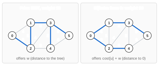
• Prim is not Dijkstra. The two share this page's code (Dijkstra.html); the only difference is the value compared. Dijkstra offers cost[u] + w (distance from the start), Prim offers just w (distance from the tree). In the example, Dijkstra from 0 keeps edge 0-1 (distance 4 either way) and builds 0-1, 0-2, 1-3, 2-4, 3-5 with weight 19, while the MST weighs 13. A shortest-path tree is generally not an MST.
• Disconnected graphs. Vertices not reachable from the start keep INF and -1, and the loop stops early (the page stops too). The result is an MST of the start vertex's component only; to get a minimum spanning forest, restart from every vertex still unknown.
• Ties. With equal weights the MST may not be unique. Different tie-breaking rules give different trees, but they all have the same total weight. If all weights are distinct, the MST is unique.
• Forgetting the known check. Updating a vertex already in the tree would overwrite its Path and break the tree.
• Negative weights are fine for Prim (unlike Dijkstra): the cut property only compares edges with each other. (This page only generates weights 1 to 9.)
• Directed graphs. "MST" of a directed graph is a different problem (minimum arborescence, Chu-Liu/Edmonds). Prim needs undirected edges.
• Kruskal's algorithm (Kruskal.html) also relies on the cut property, but sorts all edges and adds each one that does not close a cycle, using union-find: O(m log m), a natural choice for sparse graphs or edge lists, and it produces a spanning forest automatically.

Where it is used

• Designing cheap networks: cables, pipelines, road or electrical grids, circuit wiring.
• As a subroutine: the MST gives a 2-approximation for the metric travelling salesman problem, and is used in Steiner-tree heuristics.
• Clustering: removing the k − 1 heaviest MST edges gives single-linkage clusters; also image segmentation.
• Generating random mazes (Prim's algorithm with random weights).

References

Prim's algorithm

Minimum spanning tree