The idea: two greedy ways to the same minimum weight
A minimum spanning tree (MST) of a connected, weighted, undirected graph is a set of edges that connects every vertex, has no cycle, and has the smallest possible total weight. With n vertices it always has n − 1 edges.
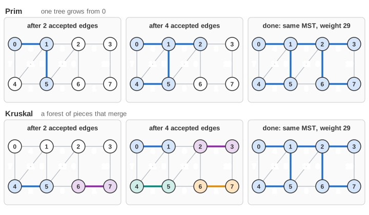
Both panels show the same graph. Prim runs on the left, Kruskal on the right, at the same time: every step of the animation examines one edge on each side. When one finishes it waits for the other. At the end the page compares the two results.
Why greedy works: the cut property
Split the vertices into two groups. That split is a cut. The cheapest edge crossing the cut is always safe: some minimum spanning tree contains it. Both algorithms only ever add such an edge. They differ in which cut they look at.
- Prim: the cut is "the tree so far | every other vertex". The cheapest edge leaving the tree is safe.
- Kruskal: it takes the globally cheapest edge not yet tried. If its ends are in two different components, it is the cheapest edge leaving either of them, so it is safe.
Prim: one tree and a priority queue
Prim starts at a start vertex (filled blue) and grows one tree. Its priority queue holds edges leaving the tree, cheapest first (light blue on the canvas, the boxes under the left graph). One step pops the cheapest entry:
- If the far end is new, the edge joins the tree (thick blue) and the new vertex's edges to non-tree vertices are pushed.
- If the far end is already in the tree, the entry is stale: it was pushed before that vertex joined. It is thrown away and counted as rejected.
This is lazy Prim: it never removes or updates queue entries, it just skips stale ones when they come up. Eager Prim keeps at most one entry per vertex (its cheapest connection) and lowers it with decrease-key, as on the Prim page. Both build the same tree.
Kruskal: sorted edges and union-find
Kruskal sorts all edges by weight once, then walks the list with a cursor (the boxes under the right graph). Each vertex starts as its own component. For each edge it asks the union-find structure for find(u) and find(v), the roots of the two ends:
- Different roots: the edge joins two components.
unionthem (the smaller root points to the bigger one) and accept the edge. The merged component takes one colour. - Same root: the edge would close a cycle. Reject it (grey, "✗ cycle").
The row of cells is the parent[] array. A root has parent[i] = i. find uses path compression: every vertex on the way is pointed straight at the root, so the cells change during a find too. So Kruskal grows a forest of many small trees that merge, while Prim grows one tree that never splits.
What the demos show
| Demo | What you see |
|---|---|
| sparse graph | 22 edges, all weights distinct. Prim needs 16 steps (14 accepted, 2 stale), Kruskal 20 (14 accepted, 6 cycles). Both weigh 177 and are the same tree. |
| dense graph | All 38 edges. Both examine 29 edges and reject 15. Prim ends with 9 stale entries still in its queue, never popped. Both weigh 130, same tree. |
| equal weights, different trees | Weights 1 or 2. Prim examines 22 edges (8 stale), Kruskal 16 (2 cycles). Both weigh 19, but 5 edges differ: Prim took 2–7, 6–10, 6–11, 7–12, 8–12; Kruskal took 2–3, 2–8, 3–4, 5–10, 5–11. |
| disconnected, tree vs forest | Two components. Prim stops after 9 steps: its queue is empty, 6 of 15 vertices, weight 86. Kruskal goes through all 21 edges (13 accepted, 8 cycles): a forest of 2 trees, weight 157, whose left tree also weighs 86. |
| long cheap chain | The 14 weight-1 edges are the whole MST (weight 14). Both finish in 14 steps with no rejection. Prim walks along the snake; Kruskal builds pieces of it that join up. |
| heavy bridge between clusters | The bridge 6–7 weighs 40, more than any other edge. Prim must cross it as soon as the left cluster is done (step 9). Kruskal reaches it last, at step 25, after 11 cycles. Both weigh 200. |
| Prim from the middle vertex | The sparse graph again, Prim starting at vertex 7: 18 steps (4 stale) instead of 16, but exactly the same tree, weight 177. Kruskal does not depend on a start vertex. |
Ties: same weight, different trees
If all weights are distinct, the minimum spanning tree is unique, so both algorithms must find the very same edges. With equal weights there can be many minimum spanning trees. Prim breaks ties by the order edges entered its queue; Kruskal by the order of the sorted list (here: weight, then the smaller vertex number). The trees can then differ, but the total weight is always the same. The edges that are in one tree and not the other pulse red at the end (Demo: equal weights, different trees).
Disconnected graphs: a spanning forest
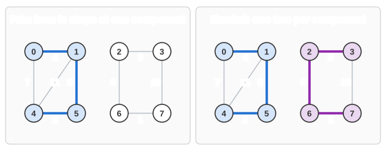
A graph with several components has no spanning tree. Prim only ever crosses edges that leave its tree, so it stops when its queue runs dry, having spanned only the start vertex's component. Kruskal does not care: it simply goes through all the edges and ends with one tree per component, a minimum spanning forest. On the start vertex's component, its tree weighs the same as Prim's (Demo: disconnected, tree vs forest).
Cost: which one is faster?
| Prim (binary heap) | Kruskal | |
|---|---|---|
| main work | up to m pushes and pops: O(m log m) lazy, O(m log n) eager | sort m edges: O(m log m), then near-constant union-find per edge |
| needs | adjacency lists, a start vertex, a connected graph | just an edge list |
| good for | dense graphs (with an array instead of a heap: O(n²), no sort of all edges) | sparse graphs, edges already sorted, forests, distributed or external-memory settings |
| can stop early | when all vertices are in the tree | after n − 1 accepted edges |
The step counter here counts edges examined, which is the honest unit of work: one heap pop for Prim, one pair of finds for Kruskal. Kruskal also pays for the full sort before its first step; Prim pays a push for each edge it discovers.
What the page leaves out
- Eager Prim with decrease-key, and Prim with a Fibonacci heap (O(m + n log n)): see Prim.
- The sort itself: Kruskal's list is shown already sorted.
- Borůvka's algorithm, which merges every component with its cheapest outgoing edge in rounds, and the linear-time randomized MST algorithm.
- Directed graphs: their analogue, the minimum spanning arborescence, needs a different algorithm (Chu–Liu/Edmonds).
See also Prim, Kruskal and Disjoint Sets (union-find), each on its own.