Splay trees: a search tree that reorganizes itself
A splay tree (Daniel Sleator and Robert Tarjan, 1985) is an ordinary binary search tree (smaller keys to the left, larger to the right) with one extra habit: every time a node is accessed, it is moved to the root by a sequence of rotations called splaying. There is no balance rule and nothing extra is stored in the nodes: no heights (as in AVL trees) and no colours (as in red-black trees).
Balanced trees guarantee O(log n) for every operation by never letting the tree get tall. A splay tree lets it get tall, but each time a long path is used, splaying roughly halves the depth of every node on it. The result is O(log n) amortized time per operation: a single operation can be slow, but any sequence of m operations costs O(m log n). Better still, frequently used keys stay near the root, so a splay tree automatically adapts to the access pattern, which a balanced tree cannot do.
The three splay steps
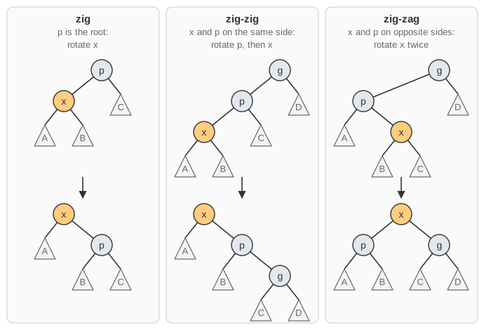
Splaying node x repeats one of three steps until x is the root. Let p be its parent and g its grandparent. The mirror-image cases work the same way; this page names each step after the direction of rotation, for example "Zig Right" and "Zig-Zig Left". Capital letters are subtrees.
zig: p is the root (one rotation, only ever as the last step)

        p                x
       / \              / \
      x   C     =>     A   p
     / \                  / \
    A   B                B   C

zig-zig: x and p are both left children (or both right children)
         rotate p above g first, then x above p

          g              x
         / \            / \
        p   D          A   p
       / \      =>        / \
      x   C              B   g
     / \                    / \
    A   B                  C   D

zig-zag: x is a right child and p a left child (or the reverse)
         rotate x above p, then x above g

          g                x
         / \             /   \
        p   D    =>     p     g
       / \             / \   / \
      A   x           A   B C   D
         / \
        B   C
splay(x):
    while x is not the root:
        p = x.parent;  g = p.parent
        if g is null:
            rotate(x)                   // zig
        else if x and p are both left or both right children:
            rotate(p); rotate(x)        // zig-zig
        else:
            rotate(x); rotate(x)        // zig-zag
The zig-zig order matters. Rotating x up twice (the simple "move to root" rule) also brings x to the root, but it can leave the path as long as it was, and a bad sequence then costs Θ(n) per access forever. Rotating the grandparent first folds the path in half.
Find, insert and delete
find(k):     search for k as in any BST
             splay the node where the search ended
             (the node with key k, or the last node visited if k is missing)

insert(k):   insert k as a new leaf, as in any BST (this page sends equal keys right)
             splay the new node to the root

delete(k):   find(k): now k is at the root (if it is in the tree)
             remove the root, leaving subtrees L and R
             if L is empty: the root is R
             else: splay the largest node of L to the top of L
                   (it now has no right child)
                   attach R as its right child
Splaying after an unsuccessful search is essential: the search already paid for walking the path, and splaying is what makes that walk pay off later.
What the animation shows
The page offers Insert, Delete, Find and Print (an in-order walk that lists the keys in sorted order), plus Insert Random, which builds a new tree from a chosen number of random keys shown in a strip below the tree (tick Random to fill the Insert box with random keys). A highlight circle follows the search path; then the message line names each splay step ("Zig Right", "Zig-Zig Left", "Zig-Zag Right", and so on) while the two or three nodes involved are rearranged. Large trees are zoomed out to fit the canvas.
Worked example
Insert 50, 30, 70, 20, 40, then delete 40, then find 60 (which is not in the tree). These are the trees the page draws.
insert 50     50

insert 30     30 becomes 50's left child; zig:
                30
                  \
                   50

insert 70     path 30 -> 50 -> 70, both right children; zig-zig:
                    70
                   /
                 50
                /
              30

insert 20     path 70 -> 50 -> 30 -> 20.
              zig-zig at 50 (20 and 30 are left children), then zig at 70:
              20
                \
                 70
                /
              30
                \
                 50

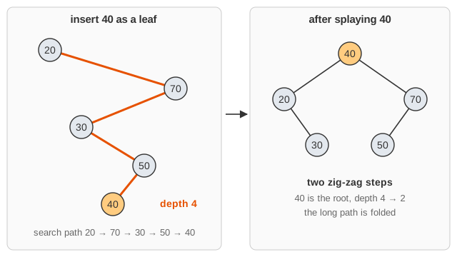
insert 40     path 20 -> 70 -> 30 -> 50 -> 40 (40 is 50's left child).
              zig-zag at 30 (40 is a left child, 50 a right child),
              then zig-zag at 20 (40 is 70's left child, 70 a right child):
                    40
                   /  \
                 20    70
                   \   /
                   30 50
              Depth 4 has become depth 2.

delete 40     40 is already the root. Remove it: L = 20-30, R = 70-50.
              The largest key in L is 30; splay it to the top of L (zig),
              then attach R as its right child:
                    30
                   /  \
                 20    70
                       /
                     50

find 60       60 > 30, go right; 60 < 70, go left; 60 > 50, but 50 has
              no right child: not found. Splay 50 (zig-zag at 30):
                    50
                   /  \
                 30    70
                /
              20
After the failed search, the keys near 60 are at the top, which is exactly what makes a following search nearby cheap.
Why it works: the amortized analysis
Give every node x a rank r(x) = lg s(x), where s(x) is the number of nodes in its subtree, and let the potential be Φ = ∑ r(x) over all nodes. A tall, path-like tree has high potential, a bushy one low potential. The Access Lemma says that each zig-zig or zig-zag step costs at most 3(r′(x) − r(x)) amortized, and the final zig at most 3(r′(x) − r(x)) + 1, where r′ is the rank after the step. Adding the steps, the sum telescopes: splaying x in a tree with root t costs at most
3 (r(t) - r(x)) + 1 ≤ 3 lg n + 1 = O(log n) amortized
Intuitively, a long access path lowers the potential by a lot (the path is folded up), and that drop pays for the long walk. Insert and delete add only O(log n) potential beyond their splays. So m operations on a tree of up to n nodes take O((m + n) log n) in total. Splay trees also satisfy stronger properties: a key accessed often is cheap (static optimality, working-set property), and accessing all keys in sorted order takes only O(n) in total. Whether they are within a constant factor of every possible BST algorithm is the famous open dynamic optimality conjecture.
Running time
operation            splay tree          splay tree        AVL / red-black
                     (amortized)         (one operation)   (worst case)
find                 O(log n)            O(n)              O(log n)
insert               O(log n)            O(n)              O(log n)
delete               O(log n)            O(n)              O(log n)
extra space / node   none                                  height or colour
A single operation can be slow: inserting 1, 2, 3, …, n in increasing order is cheap (each new key is simply rotated up once), but it leaves a path of length n, so the next find(1) walks all of it. That long walk is then paid for by the folding it causes.
Common mistakes and edge cases
- Zig-zig done as two rotations of x. That is move-to-root, which does not have the logarithmic bound. Rotate the parent first.
- Not splaying on a miss, or on delete. Every access must splay the deepest node it touched, or the analysis breaks.
- Reads change the tree. A find rewrites pointers, so splay trees are awkward to share between threads, and read-only copies cannot be used.
- Recursion depth. The tree can be Θ(n) deep, so recursive code can overflow the stack; iterative or top-down splaying avoids this.
- Duplicates need a rule: this page sends equal keys to the right subtree.
- Deleting or finding in an empty tree does nothing; deleting a missing key only splays the last node on the search path.
Variants
- Top-down splaying splays while searching down, with no parent pointers and a single pass.
- Semi-splaying moves the node only part of the way up, doing fewer rotations.
- Link-cut trees (also Sleator and Tarjan) are built from splay trees and maintain a forest of rooted trees under link and cut operations; they give fast max-flow algorithms.
- Other adaptive or randomized BSTs: treaps, skip lists and tango trees.
Where splay trees are used
Because recently used items drift to the top, splay trees work well as caches and lookup tables with skewed or bursty access patterns. They have been used in the GCC compiler (the libiberty splay-tree library), in the Windows NT kernel for virtual memory, networking and file system bookkeeping, in the FreeBSD virtual memory system, in some memory allocators, and in some implementations of ropes and text-editor buffers, where editing near the same place over and over is common. Link-cut trees built on splay trees are used in network flow and dynamic graph algorithms.