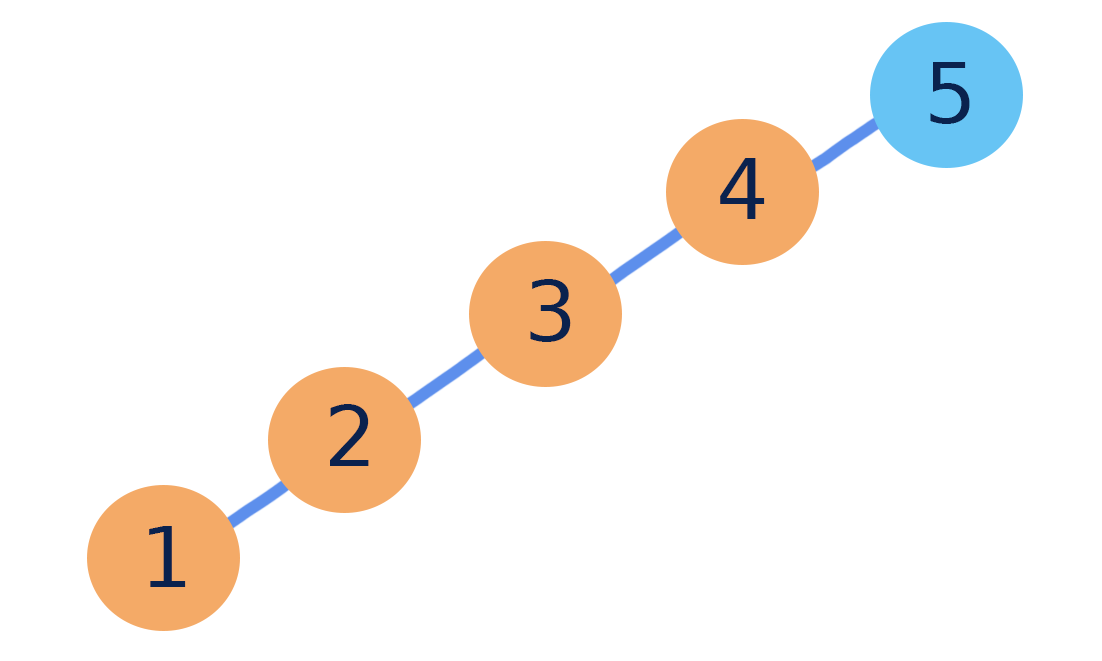
A binary search tree (BST) is a binary tree where every node in the left subtree is less than the root, and every node in the right subtree is of a value greater than the root. The properties of a binary search tree are recursive: if we consider any node as a “root,” these properties will remain true.
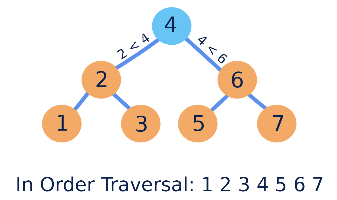
Due to the way nodes in a binary search tree are ordered, an in-order traversal (left node, then root node, then right node) will always produce a sequence of values in increasing numerical order.
Searching
Binary search trees are called “search trees” because they make searching for a certain value more efficient than in an unordered tree. In an ideal binary search tree, we do not have to visit every node when searching for a particular value.
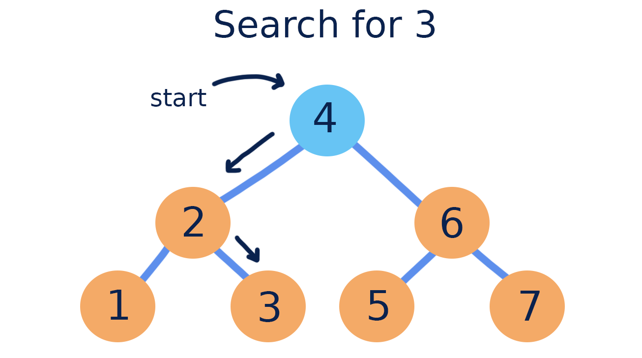
Here is how we search in a binary search tree:
- Begin at the tree’s root node
- If the value is smaller than the current node, move left
- If the value is larger than the current node, move right
Inserting
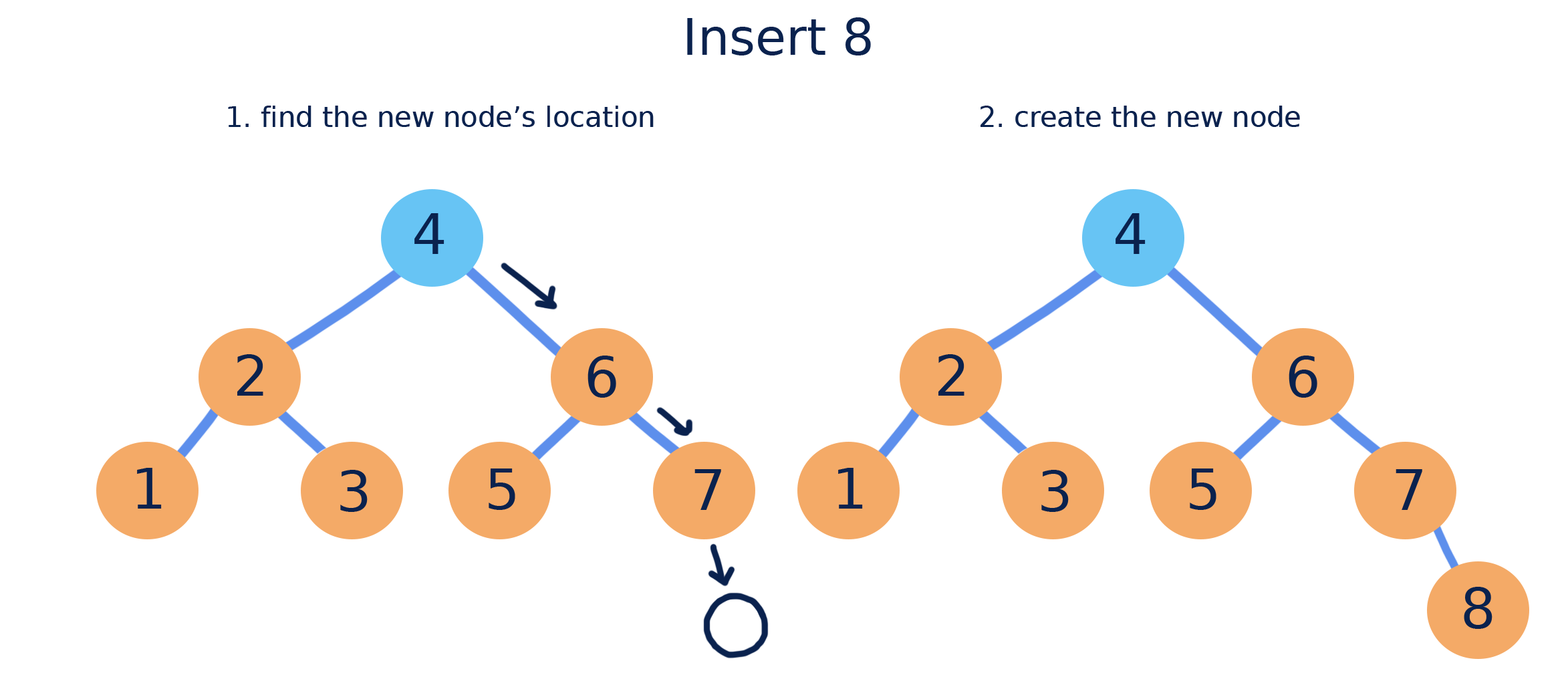
New nodes in a binary search tree are always added at a leaf position. Performing a search can easily find the position for a new node.
Removing
When removing from a binary search tree, we are concerned with keeping the rest of the tree in the correct order. This means removing is different depending on whether the node we are removing has children. There are three cases:
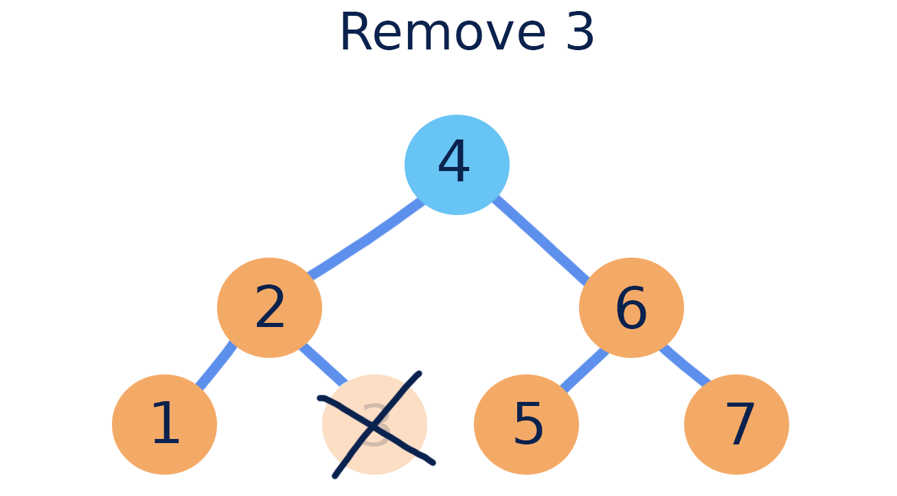
If the node being removed is a leaf, it can simply be deleted.
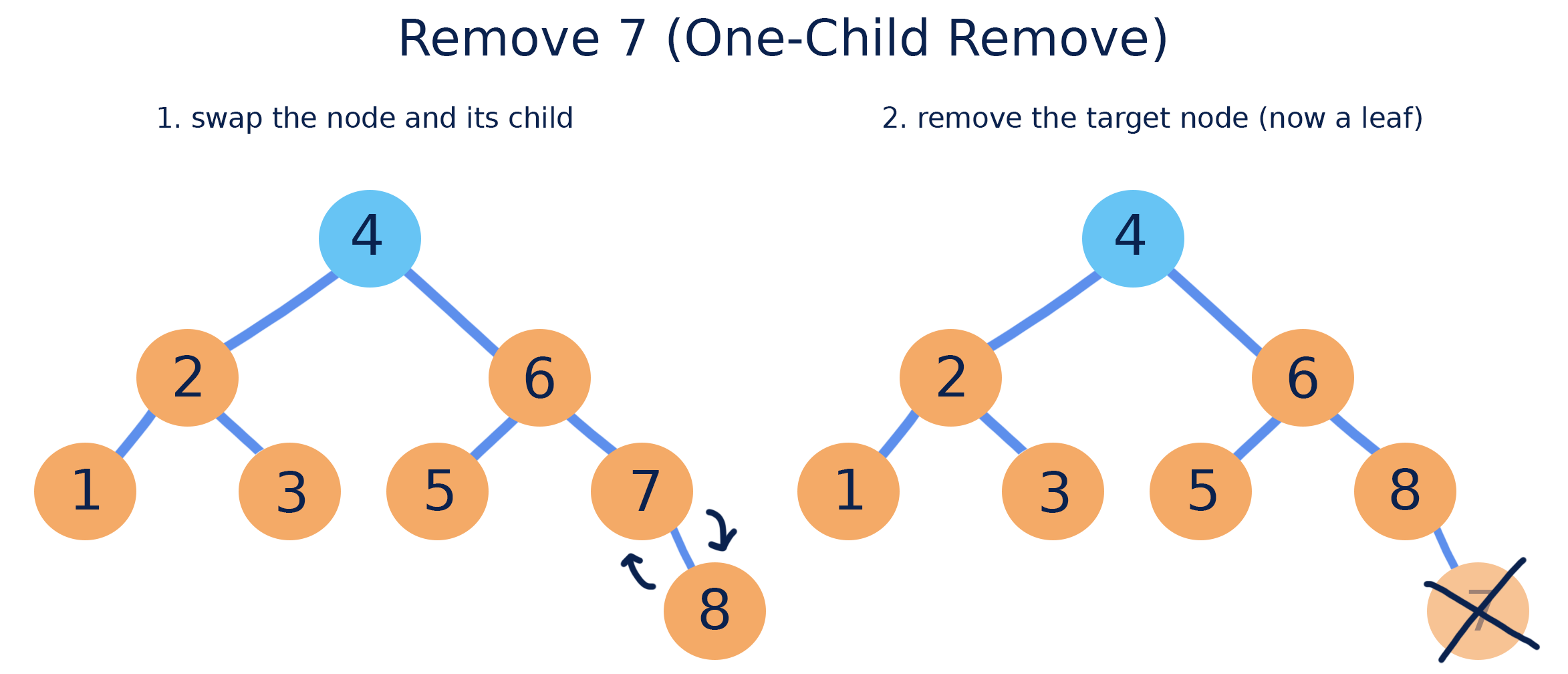
If the node has a single child, (left or right) we must move the child into the position of the node when deleting it.
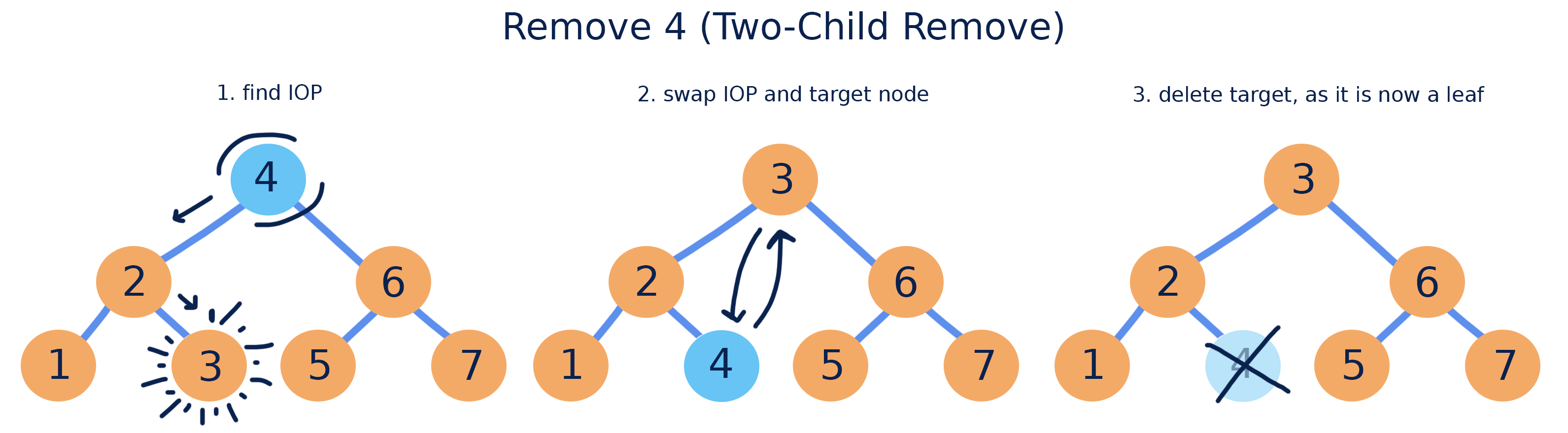
If the node has two children, we must first find the In-Order Predecessor (IOP): the largest node in our node’s left subtree. The IOP is always a leaf node, and can be found by starting at the left subtree’s root and moving right. We can then swap the node being removed with its IOP and delete it, as it is now a leaf.
Runtime and BSTs
Depending on the values contained in a binary search tree, and the order in which they are added, the performance of a BST’s operations can vary. This performance depends on the shape of the tree and the number of nodes it contains.
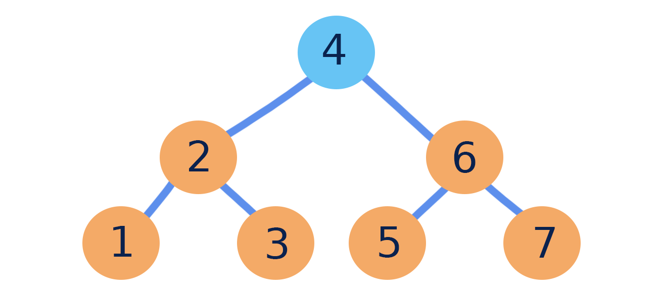
In an ideal case, a binary search tree has a similar number of nodes in its right and left subtrees. Since you have to visit less nodes when searching in an ideal BST, this case has a run time of O(lg(n)) for all operations that utilize find, including search, insert, and remove.
The worst case of a binary search tree is one that has its values added in numerical order. This structure then doesn’t resemble a tree - it looks like a linked list! As potentially every node has to be visited when searching, the worst case BST has a run time of O(n) for all operations utilizing find.