Bucket sort
Bucket sort works when the keys are numbers spread fairly evenly over a known range, for example integers 0–999 or real numbers in [0, 1). It splits the range into n equal intervals called buckets, drops every item into the bucket for its interval, sorts each bucket (they are small), and finally joins the buckets together in order. If the input is spread out evenly, each bucket holds about one item, so the whole sort takes O(n) time on average.
The idea in plain words
Think of sorting a pile of exam papers by student number. You first put them on ten piles, 0–99, 100–199, and so on, without caring about the order inside a pile. Then you tidy up each small pile, and finally you stack the piles on top of each other. Every paper in pile 3 is smaller than every paper in pile 4, so once each pile is sorted, the stack of piles is sorted too. The distribution step costs a single pass, and if the piles are small, sorting them is cheap.
What the animation shows
The page sorts n = 30 random integers below 1000 (the top row, with indices in blue). The bottom row is an array of 30 buckets. Each bucket is a pointer to a linked list, and an empty bucket is drawn with a null slash. For each value in turn, the page shows the bucket computation
index = ⌊ value × n / (MAX + 1) ⌋ = ⌊ value × 30 / 1000 ⌋
A blue circle moves to that bucket, and the value is inserted into the bucket's list in sorted order. The node it is compared with is highlighted, and the lists grow upwards from the bucket array. When all values have been distributed, the buckets are emptied from bucket 0 to bucket 29, taking each list from front to back. The values go back into the top row, and every cell that has been filled turns green.
The algorithm step by step
BucketSort(A[0..n-1], MAX):          // 0 ≤ A[i] ≤ MAX
    B[0..n-1] = n empty linked lists
    for i = 0 to n-1:                          // 1. distribute
        b = floor(A[i] * n / (MAX + 1))
        SortedInsert(B[b], A[i])
    j = 0
    for b = 0 to n-1:                          // 2. concatenate
        for each x in B[b], front to back:
            A[j] = x;  j = j + 1

SortedInsert(list, x):                        // as on this page
    if list is empty or list.head ≥ x:
        put x at the front
    else:
        p = list.head
        while p.next != null and p.next < x:
            p = p.next
        insert x after p
Dividing by MAX + 1, not MAX, makes sure that even the largest possible value gets an index below n: ⌊999 × 30 / 1000⌋ = 29. The formula keeps the order of values: if x ≤ y, then bucket(x) ≤ bucket(y). Inserting each value into its place in the list is insertion sort done one item at a time. Many textbooks instead append to the bucket and sort each bucket at the end, which gives the same result.
A worked example
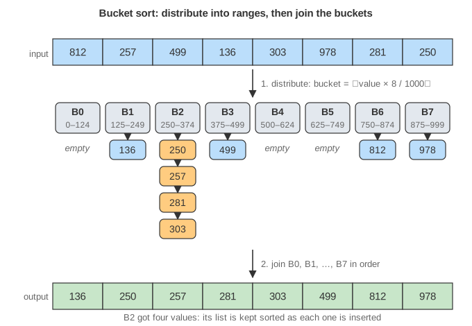
The same scheme with n = 8 values and MAX = 999, so that index = ⌊value × 8 / 1000⌋. The input is 812 257 499 136 303 978 281 250.
value  value*8/1000   bucket  what happens                         bucket afterwards
812      6.496          6     bucket empty                         6: 812
257      2.056          2     bucket empty                         2: 257
499      3.992          3     bucket empty                         3: 499
136      1.088          1     bucket empty                         1: 136
303      2.424          2     257 < 303, end of list: after 257    2: 257 → 303
978      7.824          7     bucket empty                         7: 978
281      2.248          2     257 < 281; 303 ≥ 281: after 257     2: 257 → 281 → 303
250      2.000          2     head 257 ≥ 250: at the front        2: 250 → 257 → 281 → 303
Notice that 499 goes to bucket 3 (3.992 is rounded down), and 250 lands exactly on the boundary 2.000, so it goes to bucket 2. The buckets at the end:
B0: empty          B4: empty
B1: 136            B5: empty
B2: 250 → 257 → 281 → 303    B6: 812
B3: 499            B7: 978
Concatenating B0, B1, …, B7 gives 136 250 257 281 303 499 812 978, which is sorted. Four values landed in bucket 2 and three buckets stayed empty. Even input drawn at random is never spread perfectly evenly.
Why it is correct
Take two values x < y. If they are in different buckets, then x's bucket has the smaller index, because the bucket formula never decreases as the value grows. Since buckets are joined in index order, x comes out first. If they are in the same bucket, the sorted insertion keeps that bucket's list in order, so again x comes first. So every pair ends up in the right order.
Time and space complexity
- Distribution and joining cost O(n): one bucket computation per item, plus a visit to each of the n buckets.
- Sorting inside the buckets costs O(ni2) for a bucket that gets ni items, because each insertion may walk the whole list.
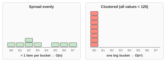
- Average case, uniform input: O(n). If each value falls into any of the n buckets with equal probability, independently of the others, then ni is binomial with n trials and probability 1/n. So E[ni2] = Var + mean2 = (1 − 1/n) + 1 = 2 − 1/n. Summing over the n buckets, the expected sorting work is n(2 − 1/n) = 2n − 1 = O(n). The buckets are small on average, and large buckets are rare enough that their quadratic cost does not add up.
- Worst case: Θ(n2). If all values fall into one bucket, the algorithm is simply insertion sort. On this page every value from 0 to 33 goes to bucket 0 (⌊33 × 30/1000⌋ = 0), so 30 values all below 34 would give one bucket with 30 items. Clustered or skewed input (such as exponential or "mostly small" values) causes the same problem. Sorting each bucket with an O(m log m) sort instead brings the worst case down to O(n log n).
- Space: O(n) extra, for the n bucket heads and n list nodes. It is not in-place.
Common mistakes, edge cases and variants
- Index out of range. Writing
value * n / MAXsends the maximum value to bucket n, which does not exist. For real keys in [0, 1), usefloor(x * n). For a range [min, max], usefloor((x − min) * n / (max − min + 1)). This also handles negative keys. - Using the wrong range. The range must be known, or found in a first pass. If a few huge outliers stretch the range, nearly everything else crowds into the first buckets.
- Stability. The insertion on this page puts a new value before any equal values already in the bucket (it stops at the first element ≥ the new one). Equal keys therefore come out in reverse input order, so this version is not stable. That does not matter for plain numbers, but for records you should insert after equal keys (stop at the first element > the new one), or append and then sort each bucket stably.
- Number of buckets. Using n buckets keeps the expected bucket size at 1. Far fewer buckets make each one bigger. Far more buckets waste time and memory on empty ones.
- Related sorts. With one bucket for every possible integer key, bucket sort becomes counting sort. Distributing by one digit at a time and repeating gives radix sort.
Where it is used
- Sorting values that are roughly uniform, such as random floating-point numbers, hash values and sensor readings over a known range.
- Histograms and "binning" in data analysis and graphics, and spatial hashing into grid cells in games and simulations.
- Parallel and external sorting: in "sample sort", splitters chosen from a sample define buckets that different machines or disks sort on their own.