Counting Sort Visualization

Counting sort

Counting sort sorts n items whose keys are small non-negative integers, say in the range 0, 1, …, k. It never compares two keys with each other. Instead it uses each key as an array index: it counts how many times every key occurs, turns those counts into positions, and then writes every item straight into its final place. Because it does not compare, it is not bound by the Ω(n log n) lower bound that holds for comparison sorts such as merge sort or heap sort, and it runs in O(n + k) time.

The idea in plain words

Suppose a teacher has 30 exam papers graded 0 to 30 and wants them in order. She could compare papers two at a time, but it is faster to count: "one paper got 0, three got 1, none got 2, …". If three papers got a grade of 1 or less, then the papers with grade 1 go in places 1, 2 and 3 of the sorted pile (counting from 0, after the one paper with grade 0). In general, the number of items with key ≤ v tells you where the block of key v ends in the output. Adding up the counts from left to right (a prefix sum) gives exactly those numbers.

What the animation shows

The page sorts 30 random integers. The top row is the input array (indices 0–29 in blue under the cells). The middle row is the count array C with one cell for every possible key 0–30. The bottom row is the output array. The animation goes through three phases:

1. Count. A blue circle travels from each input cell to the count cell for its key, and that count goes up by 1. Input cells that have been counted fade out.
2. Prefix sums. Neighbouring count cells C[i-1] and C[i] are highlighted, and C[i] becomes C[i] + C[i-1].
3. Place. Going through the input from the last cell to the first, a blue circle goes to the key's count cell, the count is decreased by 1, and a light-blue circle goes from there to that index in the output array. The value moves down and its output cell turns green. At the end the sorted output is copied back into the top row.

The algorithm step by step

CountingSort(A[0..n-1], k):          // every key is in 0..k
    C[0..k] = all 0
    for i = 0 to n-1:                // 1. count
        C[A[i]] = C[A[i]] + 1
    for v = 1 to k:                  // 2. prefix sums
        C[v] = C[v] + C[v-1]         //    now C[v] = number of keys ≤ v
    for i = n-1 downto 0:            // 3. place, right to left
        C[A[i]] = C[A[i]] - 1
        B[C[A[i]]] = A[i]
    copy B back into A

After step 2, C[v] is one past the last position of the block of key v. In step 3 each item first decreases its key's counter and then goes to that index, so the items of key v fill their block from its right end towards its left end. This is exactly what the page's code does (insertIndex = --C[A[i]]).

A worked example

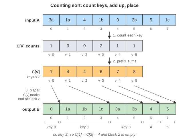
Sort A = 3 1 4 1 0 3 5 1 (n = 8, keys 0…5, so k = 5). To follow stability, the equal keys are tagged in the order they appear: 3a 1a 4 1b 0 3b 5 1c.

1. Count. Key 0 occurs once, key 1 three times, key 2 never, key 3 twice, keys 4 and 5 once each:

v       0  1  2  3  4  5
C[v]    1  3  0  2  1  1

2. Prefix sums. C[1] = 3 + 1 = 4, C[2] = 0 + 4 = 4, C[3] = 2 + 4 = 6, C[4] = 1 + 6 = 7, C[5] = 1 + 7 = 8:

v       0  1  2  3  4  5
C[v]    1  4  4  6  7  8     C[v] = how many keys are ≤ v

Read it as block boundaries: key 0 goes in position 0, keys 1 in positions 1–3, no key 2, keys 3 in 4–5, key 4 in 6, key 5 in 7.

3. Place, from right to left.

i  A[i]  C[A[i]] before → after   write          C after
7   1c        4 → 3              B[3] = 1c      1 3 4 6 7 8
6   5         8 → 7              B[7] = 5       1 3 4 6 7 7
5   3b        6 → 5              B[5] = 3b      1 3 4 5 7 7
4   0         1 → 0              B[0] = 0       0 3 4 5 7 7
3   1b        3 → 2              B[2] = 1b      0 2 4 5 7 7
2   4         7 → 6              B[6] = 4       0 2 4 5 6 7
1   1a        2 → 1              B[1] = 1a      0 1 4 5 6 7
0   3a        5 → 4              B[4] = 3a      0 1 4 4 6 7

B = 0 1a 1b 1c 3a 3b 4 5

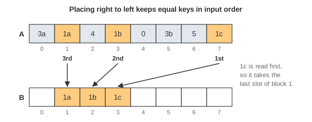
The three 1s come out as 1a 1b 1c and the two 3s as 3a 3b: the same order as in the input. Notice also that at the end C[v] holds the first position of each block (C[3] = 4, where 3a went).

Why it is correct, and why it is stable

• Every item gets its own slot. Before step 3 the counter of key v points just past a block of exactly count(v) free slots, and the blocks of different keys do not overlap. Each item of key v takes the next slot to the left inside its own block, and there are exactly as many items as slots, so no slot is written twice and none stays empty.
• The output is sorted. All slots of key v lie before all slots of any larger key, because the blocks are laid out in key order by the prefix sums.
• It is stable: items with equal keys keep their input order. Inside a block the slots are filled from right to left, and the input is also read from right to left. So the last item with key v gets the last slot of the block, the one before it gets the slot before, and so on.

Stability does not matter when you sort plain numbers, because two equal 1s look the same. It matters a lot when the key is only part of a record, and above all in radix sort. Radix sort sorts numbers digit by digit, from the least significant digit to the most significant, with counting sort on one digit (k = 9) in each pass. Each pass must be stable, or it destroys the order that the earlier passes built. For example, sort 13 12: the ones pass gives 12 13. In the tens pass both numbers have tens digit 1. A stable pass keeps 12 13, which is correct. An unstable pass is allowed to swap them and gives 13 12, which is wrong.

Time and space complexity

• Clearing C and the prefix-sum loop each take O(k). The counting loop, the placing loop and the copy back each take O(n). So the total is Θ(n + k) in every case: best, average and worst. The input order does not matter.
• Extra space: O(k) for C plus O(n) for the output B. Counting sort is not in-place.
• This is linear when k = O(n), as on this page (30 keys in 0–30). It is a bad idea when the key range is large compared with n. Sorting 10 phone numbers with 10 digits would need a count array of 10¹⁰ cells, and nearly all of the time would go into clearing and scanning empty counters. For large ranges, use radix sort (several counting passes over small digits) or a comparison sort.

Common mistakes, edge cases and variants

• Placing from left to right with this code. If you decrease-then-place while scanning from left to right, equal keys come out in reverse order and the sort is no longer stable. The result is still sorted, but using it inside radix sort gives wrong answers. The left-to-right variant must first turn C into starting positions (C[v] = number of keys < v), and then place-then-increase.
• Off-by-one errors. C needs k + 1 cells for keys 0…k. On this page there are 31 cells for keys 0–30. Decreasing after writing instead of before writes one slot too far to the right.
• Negative keys or keys that do not start at 0. Shift by the minimum: use index A[i] − min, so that the array has max − min + 1 cells.
• Sorting records. Count on the key but move the whole record. This is where stability pays off.
• Simple counting variant. For bare integers with no attached data, you can skip the prefix sums and the output array: after counting, write key v C[v] times for each v. This is still O(n + k), but it only works when the keys are the whole data.
• Counting sort with many buckets instead of exact keys is bucket sort.

Where it is used

• As the stable inner pass of LSD radix sort, for integers, fixed-length strings, IP addresses and dates.
• Sorting by a small key: grades, ages, days of the week, letters, pixel intensities 0–255 (building image histograms is the counting phase on its own).
• Building suffix arrays and doing parallel "bucketing" on GPUs, where the prefix sum (scan) step works very well in parallel.

References

Counting sort (Wikipedia)