Quick Sort vs Merge Sort
This page builds one array, copies it twice, and runs Quick Sort on the top copy and Merge Sort on the bottom copy at the same time, one comparison at a time. Both are divide-and-conquer sorts that take about n log₂ n comparisons on a typical array. What the page is really about is the other two scoreboards: how much extra memory each one needs while it works, and how long each one actually takes.
Pick the number of items (20 to 60) and the initial order, press Sort Both, and watch four things: the bars, the stack of calls drawn under each array, the buffer row that only Merge Sort uses, and the two pairs of meters at the bottom.
Same idea, opposite order
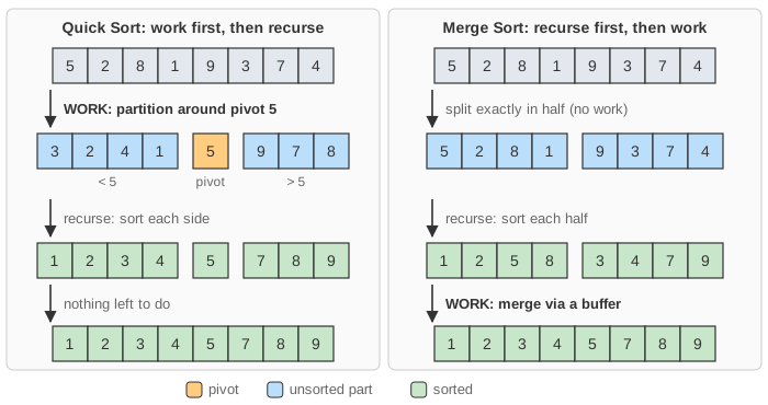
Both split the array, sort the pieces recursively, and are done when the pieces are sorted. They differ in when the real work happens:
quickSort(a, lo, hi):                        mergeSort(a, lo, hi):
    if lo >= hi: return                          if lo >= hi: return
    p = partition(a, lo, hi)   <-- work          mid = (lo + hi) / 2
    quickSort(a, lo, p - 1)                      mergeSort(a, lo, mid)
    quickSort(a, p + 1, hi)                      mergeSort(a, mid + 1, hi)
                                                 merge(a, lo, mid, hi)   <-- work

partition: pivot = a[lo]; i scans right       merge: repeatedly take the smaller front
  past values < pivot, j scans left past        value of the two sorted halves into a
  values > pivot, swap a[i] and a[j];           buffer, then copy the buffer back into
  when they cross, swap the pivot into a[j].    a[lo..hi].
Quick Sort does its work before recursing, in place, by swapping. Where the split lands depends on the pivot, so the two halves can be very unequal. Merge Sort splits exactly in half without looking at the data, and does its work after recursing, and merging two sorted runs is only easy with somewhere else to put the result.
Counting comparisons
- Merge Sort merges runs of total length k with at most k − 1 comparisons, and every value takes part in about log₂ n merges. Its worst case is at most n⌈log₂ n⌉ − n + 1 comparisons, whatever the input. On already-sorted input it does even fewer, because one half runs out early.
- Quick Sort averages about 1.39 n log₂ n comparisons on random input, a little more than Merge Sort. Its worst case is ≈ n² / 2, when every pivot is the smallest or largest value left. With the first element as the pivot, already sorted input is exactly that case.
This page's own numbers, averaged over 250 arrays each:
                         comparisons              peak extra memory (cells)
                    Quick Sort   Merge Sort       Quick Sort   Merge Sort
25 items, random         106           87              7.3          26
60 items, random         346          281             10.1          61
60 items, sorted        1749          184             56.4          61
60 items, reversed      1160          181             37.4          61
60 items, few unique     298          270              7.9          61
Counting memory
The page counts extra memory in cells. One cell is one stack frame (a recursive call that is still running) or one slot of a temporary buffer. The array being sorted isn't counted, since both sorts need that.
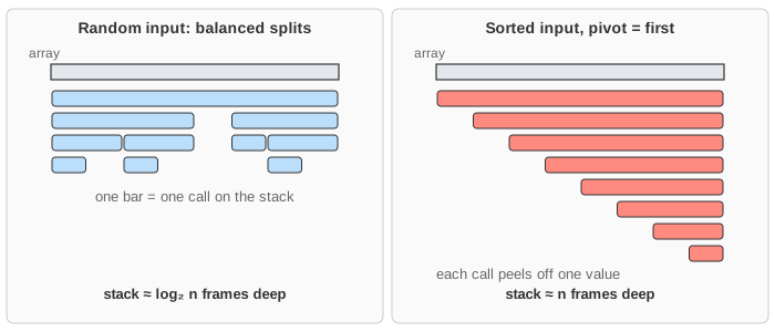
- Quick Sort sorts in place, so its only extra memory is the recursion stack. Each running call is drawn as a bar under the part of the array it is working on, one row per level. On a random array the stack stays around log₂ n deep. On sorted input every partition peels off one value and the stack grows almost n deep: O(n) extra memory, which is how real programs hit a stack overflow. The standard fix is to recurse into the smaller side and loop on the larger one. That caps the stack at log₂ n frames, whatever the pivots.
- Merge Sort needs the same shallow stack (⌈log₂ n⌉ levels) plus a buffer as large as the range it is merging. On the final merge that is the whole array, so its peak is always n + 1 cells on this page, on every input. The buffer row fills up and empties with each merge, so you can see it.
Why Quick Sort is usually faster anyway
Comparisons are not the whole cost. Quick Sort does its swaps inside one array that stays in the CPU cache. Merge Sort copies every value into the buffer and back on every level, which roughly doubles the memory traffic. So in practice a well-implemented Quick Sort, with a random or median-of-three pivot, usually finishes first despite its extra comparisons. That is why C's qsort and C++'s std::sort are Quick Sort variants (introsort).
The Finish time meters test this directly. When you press Sort Both, the page first runs both sorts on this array in your browser without any animation, repeating each thousands of times, since one sort of 60 values takes only microseconds. It reports the time per sort from the fastest of five batches. Try Already sorted with 60 items: Quick Sort makes about nine times as many comparisons and still finishes in about the same time. Its inner loop only steps an index down a row of numbers the CPU predicts perfectly, while Merge Sort allocates a buffer for every merge and copies every value twice. These are real measurements, so they change a little from run to run and from browser to browser. Comparisons and memory never change for the same array.
When to pick Merge Sort
- You need a guarantee. Merge Sort is O(n log n) on every input, with no bad pivots.
- You need a stable sort, where equal keys keep their original order. Merge Sort is stable if it takes from the left half on ties (this page does:
≤). Quick Sort is not. This is why Java sorts objects with a merge-sort variant (TimSort), as does Python'ssorted. - Linked lists. Merging two lists needs no buffer at all, just relinking.
- Data larger than memory. Merging sorted runs streams from disk sequentially: see the external merge sort visualizer.
What "at the same time" means here
The two sorts are stepped in lockstep by comparisons: after step k, each side has compared k pairs of values. Everything a comparison causes (a swap, a copy into the buffer, a call returning) happens in the same step. When one side finishes, its panel turns green and the other keeps going. On big or badly ordered arrays one step covers several comparisons, so a run never takes more than about 160 steps.
Common mistakes
- Always using the first element as the pivot. It is the simplest choice (and this page uses it, to show the problem), but sorted or nearly-sorted data, which is very common in practice, then costs n² / 2 comparisons and n stack frames. Try Already sorted with 60 items.
- Saying "Merge Sort is O(n log n)" and stopping there. It also needs O(n) extra memory, which matters on small devices and large arrays.
- Saying "Quick Sort needs no extra memory". It needs a stack, O(log n) on average and O(n) in the worst case unless you recurse into the smaller side first.
- Comparing on one small random array. The counts swing from array to array. Press New Random Array a few times, and try all four orders.
- Allocating a new buffer on every merge in real code. This page does it so each buffer can be drawn, but a real implementation allocates one n-cell buffer once and reuses it.