The idea: each cell is a row times a column
To multiply A by B, take row i of A and column j of B, pair their entries in order (first with first, second with second, …), multiply each pair and add the products. That sum is the entry C[i][j] of the product C = AB. It is the dot product of a row and a column:
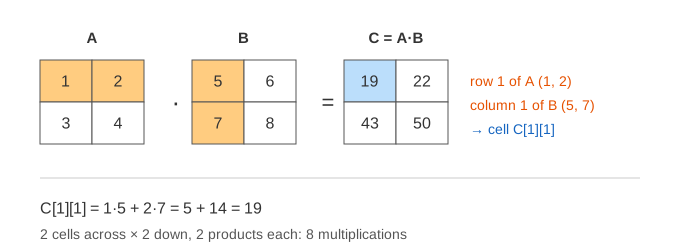
On the canvas the row and the column turn orange, the target cell of C turns blue, and each product appears on its entry of A and then flies into the term row. The sum flies into C (Demo: 2×2 product, cell by cell). For [1 2; 3 4]·[5 6; 7 8] the four cells are 1·5 + 2·7 = 19, 1·6 + 2·8 = 22, 3·5 + 4·7 = 43 and 3·6 + 4·8 = 50.
The shape rule: (m×n) · (n×p) = m×p
A row of A has as many entries as A has columns (n). A column of B has as many entries as B has rows. They can only be paired up if those two numbers are equal, so the inner sizes must match. The result takes the outer sizes: one cell for every row of A and every column of B.
| A | B | A·B |
|---|---|---|
| 2×2 | 2×2 | 2×2 |
| 2×3 | 3×2 | 2×2: each cell adds 3 products (Demo: 2×3 · 3×2) |
| 2×3 | 2×2 | undefined: 3 ≠ 2 (Demo: shape mismatch) |
| 3×2 | 2×3 | 3×3: the other order of the 2×3 · 3×2 pair is bigger |
| n×n | n×1 (a vector) | n×1: a matrix times a vector |
In the mismatch demo, row 1 of A = (1, 0, 2) has three entries but column 1 of B = (1, 3) has two, so the 2 has nothing to multiply with. Note that B·A = (2×2)·(2×3) is fine there: whether a product exists can depend on the order.
Counting the work: n³
Every cell of C needs n multiplications (and n − 1 additions), and there are m·p cells, so the schoolbook method does m·n·p multiplications. The canvas counts them: 8 for 2×2 · 2×2, 12 for 2×3 · 3×2. For two square n×n matrices that is n³: 1 000 × 1 000 matrices take a billion multiply-adds, and doubling n means eight times the work. Strassen’s trick does a 2×2 block product with 7 multiplications instead of 8, which gives about n2.81; in practice libraries keep the n³ method and make it fast with cache blocking and SIMD.
A·B means: apply B, then A
A 2×2 matrix moves the points of the plane: its first column is where (1, 0) lands, its second column is where (0, 1) lands. Applying B to a point x and then A to the result gives A(Bx). Matrix multiplication is defined exactly so that this is one matrix:
So the matrix written next to x, the right-hand one, acts first. Press Transform to see the unit square with an F move to Bx and then to A(Bx) (Demo: composition = apply B, then A). The columns of AB are where the corners (1, 0) and (0, 1) end up.
AB ≠ BA: order matters
Take a 90° rotation R = [0 −1; 1 0] and a shear S = [1 1; 0 1]. Shearing first and then rotating gives RS = [0 −1; 1 1]. Rotating first and then shearing gives SR = [1 −1; 1 0]. Different matrices, different pictures (Demo: AB ≠ BA: the grey copy keeps the first result).
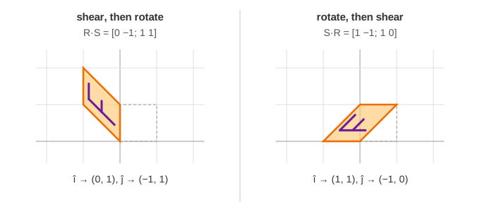
Some pairs do commute: two rotations, two scalings, any matrix with the identity or with its own inverse. But in general, swapping the order changes the result, and with non-square matrices one order may not even be defined.
Identity and inverse
The identity I = [1 0; 0 1] keeps (1, 0) and (0, 1) in place, so it moves nothing: AI = IA = A, the way 1 works for numbers. The inverse A−1 undoes A: AA−1 = A−1A = I. For A = [2 1; 1 1], A−1 = [1 −1; −1 2]; on the canvas A−1 moves the shape and A moves it straight back home (Demo: identity and inverse). An inverse exists only when det A ≠ 0 (here 2·1 − 1·1 = 1), see Determinant.
Where it shows up
- Graphics: rotate, scale and shear are matrices, and a chain of them is multiplied into one matrix before it is applied to thousands of vertices (Rotation and Scaling in 2D).
- Neural networks: a layer computes W·x + b, a matrix times a vector; a batch of inputs makes it a matrix times a matrix (Neural Network: the Forward Pass).
- Attention: the scores are QKT and the output is softmax(…)·V, two matrix products (Self-Attention).
See also 2D Vectors and the Dot Product (each cell is one dot product) and Gaussian Elimination (solving Ax = b instead of computing Ax).
Multiplying a whole chain? The order matters: see Matrix Chain Multiplication (p·q·r per product, best parenthesization by dynamic programming).
Karatsuba multiplication uses the same trick for numbers as Strassen's for matrices: one fewer half-size product.
See also NumPy Broadcasting for element-wise operations on arrays of different shapes, whose shape rule is not the (m × n)·(n × p) rule of the matrix product.
See also Cache-Friendly Loops: Traversal Order, Interchange and Tiling for how the order of the three loops and cache blocking change the number of cache misses of the same product.
What the page leaves out
Matrices stay small with whole-number entries. The page does not show the column view (each column of AB is A times a column of B), block matrices, associativity (AB)C = A(BC) and how the chosen order changes the cost of a chain, Strassen’s algorithm, cache blocking and GPUs, or floating-point rounding.