The idea: one number splits the image in two
Thresholding turns a grey image into a black-and-white one. Pick one number t. Every pixel whose level v is above t becomes white; every other pixel becomes black. On the histogram, t is a cut: the bars left of it form class 0 (black), the bars right of it form class 1 (white). The hard part is choosing t. Otsu's method chooses it from the histogram alone.
The page uses an 8×8 image (64 pixels) with 8 grey levels, 0 = black to 7 = white. Each preset image comes with its intended answer, so the page can count the wrong pixels and mark them with a red ✗. Threshold applies the t you pick, Otsu tries every t and keeps the best, and Adaptive gives every pixel a threshold of its own.
Choosing t by hand
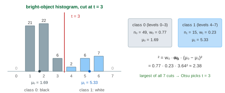
The bright object image has a blob of levels 4 to 6 on a background of levels 1 to 3. Its histogram has two humps: counts 0, 21, 22, 6 | 2, 6, 7, 0. Any cut between the humps works; a cut inside a hump moves whole bars to the wrong side.
| t | 0 | 1 | 2 | 3 | 4 | 5 | 6 |
|---|---|---|---|---|---|---|---|
| wrong pixels | 49 | 28 | 6 | 0 | 2 | 8 | 15 |
With t = 1 the 22 background pixels at level 2 and the 6 at level 3 turn white: 28 wrong (Demo 2: t = 1 is too low). With t = 5 the object pixels at levels 4 and 5 turn black: 8 wrong (Demo 3: t = 5 is too high). A point rule like this treats all pixels of one level the same, so a mistake is always a whole bar.
Otsu's method: the between-class variance
For each cut t, Otsu splits the pixels into the two classes and computes four numbers: the weights w₀ = n₀ / 64 and w₁ = n₁ / 64 (the share of pixels in each class) and the class means μ₀ and μ₁ (the average level in each class). Then:
σB²(t) = w₀ · w₁ · (μ₀ − μ₁)²
This is the between-class variance. It is large when the two means are far apart and both classes are big. Otsu picks the t with the largest value (Demo 1: Otsu finds t = 3):
| t | 0 | 1 | 2 | 3 | 4 | 5 | 6 |
|---|---|---|---|---|---|---|---|
| n₀ / n₁ | 0 / 64 | 21 / 43 | 43 / 21 | 49 / 15 | 51 / 13 | 57 / 7 | 64 / 0 |
| μ₀ | — | 1.00 | 1.51 | 1.69 | 1.78 | 2.12 | 2.55 |
| μ₁ | 2.55 | 3.30 | 4.67 | 5.33 | 5.54 | 6.00 | — |
| σB² | 0 | 1.17 | 2.19 | 2.38 | 2.28 | 1.46 | 0 |
At t = 0 and t = 6 one class is empty, so the score is 0. The best t is 3, and it gets every pixel right. Only the histogram was needed: one pass to count, then 7 short sums. If two cuts tie, the first one is kept (OpenCV does the same).
Why "between"? The total variance of the levels, σ² = 2.84 here, does not depend on t. It splits into two parts: σ² = σW² + σB², where σW² is the spread inside each class (the within-class variance). So the t with the largest σB² is also the t with the smallest σW²: the two classes are as tight as they can be. At t = 3, σW² = 2.84 − 2.38 = 0.46.
Uneven lighting: no single t works
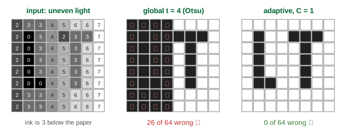
The uneven light image is paper with the letters L and T, lit from the right. The paper goes from level 2 on the left to 7 on the right, and each ink pixel is 3 levels darker than the paper next to it. The ink on the bright side (levels 2 and 3) is as light as the paper on the dark side (levels 2 to 4). So no cut can put all ink below and all paper above. The best global t still makes 7 mistakes, and Otsu picks t = 4 (σB² = 2.96), which turns 26 paper pixels on the dark side black (Demo 4: uneven light, Otsu fails).
Adaptive threshold: compare each pixel with its neighbours
An adaptive threshold gives each pixel its own cut, computed from the pixels around it. Here it is the local mean of the 3×3 window, minus a small offset C:
T(x, y) = mean of the 3×3 window around (x, y) − C white if v > T(x, y)
At the edge the window is cut to the pixels inside the image (6 or 4 of them). Ink is darker than the paper around it, so it falls below its local mean; paper sits at or above it. The light level cancels out, because it is about the same across one small window. With C = 1 every pixel is right (Demo 5: local mean threshold, C = 1). The demo looks at two pixels with the same level v = 3. The paper pixel at row 3, column 2 has window mean 21 / 9 = 2.33, so T = 1.33 and it stays white. The ink pixel at row 3, column 5 has window mean 42 / 9 = 4.67, so T = 3.67 and it turns black. A global threshold must give both the same colour.
The offset C
C says how much darker than its neighbours a pixel must be to count as ink.
| C | wrong pixels | what goes wrong |
|---|---|---|
| 0 | 8 | paper at or a little below the mean of its window (a flat patch, or the darker side of a slope) fails v > T and turns into a black speck (Demo 6: C = 0 makes specks) |
| 1 | 0 | flat paper stays white, every ink pixel is still 1 below its mean |
| 2 | 8 | ink pixels inside a stroke have ink neighbours, so they are less than 2 below the mean and turn white (Demo 7: C = 2 loses thin ink) |
The window size matters as well. It must be bigger than the strokes, or the inside of a thick shape has only its own colour around it and looks like background. Real documents use windows of 11 to 51 pixels.
Global vs adaptive
| global t (by hand or Otsu) | adaptive local mean | |
|---|---|---|
| threshold | one number for all pixels | one number per pixel |
| built from | the histogram (Otsu) or a guess | the window around each pixel, and C |
| cost | count once, then one compare per pixel | a window mean per pixel (a running sum makes it cheap) |
| works when | the histogram has two clear humps | the light changes slowly across the image |
| fails when | the light is uneven, or one class is tiny | shapes are bigger than the window; C is badly chosen |
The black-and-white result is often cleaned up next with opening and closing; see Erosion and Dilation. To spread out a dull histogram instead of cutting it, see Histogram Equalization. To find object outlines from the gradient rather than from levels, see Canny Edge Detection, which also uses two thresholds, on edge strength.
See also the Hough transform, which finds straight lines among the white pixels of a binary edge image by letting each pixel vote.
What the page leaves out
Real images have 256 levels, so Otsu tries 255 cuts; the sums are kept as running totals so the sweep stays one pass over the histogram. Multi-level Otsu cuts the histogram into three or more classes. Otsu struggles when one class is very small or the humps overlap a lot; smoothing the image first often helps. OpenCV's adaptive threshold also offers a Gaussian-weighted window (ADAPTIVE_THRESH_GAUSSIAN_C), copies edge pixels outward instead of cutting the window, and rounds the mean. Other local methods (Niblack, Sauvola) also use the local standard deviation. Colour images are usually thresholded on one channel or on brightness.
On the mind map
References
N. Otsu: A Threshold Selection Method from Gray-Level Histograms, IEEE Trans. SMC 9(1), 1979
OpenCV: Image Thresholding (simple, adaptive and Otsu's binarization)
HIPR2 (University of Edinburgh): Adaptive Thresholding
Gonzalez and Woods: Digital Image Processing, 4th ed., chapter 10 (thresholding)