The idea: follow one digit through the network
A convolutional neural network (CNN) is a chain of layers. Each layer takes a block of numbers with some shape and gives back a block with a new shape. If you can work out that shape and the number of weights for each kind of layer, you can read any CNN summary line by line. This page does it for LeNet-5, the small network that reads 28×28 handwritten digits.
The network: conv1 (6 filters of 5×5, padding 2) → max-pool → conv2 (16 filters of 5×5) → max-pool → flatten → dense 120 → dense 84 → dense 10 with softmax. This is the version in most tutorials and in the d2l.ai book. How one kernel slides over an image is on Convolution in a CNN; this page looks at the whole network at once.
Shapes: conv, pool, flatten, dense
A conv or pool layer works on maps of size W×W with C channels. With a K×K window, padding P and stride S, the new width is
out = ⌊(W − K + 2P) / S⌋ + 1
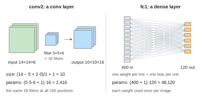
- conv: the depth becomes the number of filters. conv1: (28 − 5 + 2·2)/1 + 1 = 28, so 28×28×6.
- pool: max 2×2 with stride 2 halves the width and keeps the depth. pool1: (28 − 2)/2 + 1 = 14, so 14×14×6.
- flatten: lays the maps out in one row. 5×5×16 becomes 400 numbers.
- dense (fully connected): the output is just the number of units: 120, 84, 10.
Press Next Layer to see each step: the previous shape flies into the layer, the new shape appears, then its weights are counted (Demo 1: LeNet-5, one layer at a time).
Counting parameters
A conv filter has K·K·Cin weights and one bias, and there is one filter per output channel: (K·K·Cin + 1)·Cout. The image size is not in the formula, because the same filter is reused at every position. A dense layer has one weight per input-output pair and one bias per unit: (in + 1)·out. Pooling and flatten have no weights.
| layer | output | parameters | multiply-adds |
|---|---|---|---|
| input | 28×28×1 | 0 | 0 |
| conv1 5×5, 6, P 2 | 28×28×6 | (5·5·1 + 1)·6 = 156 | 117,600 |
| pool1 2×2, S 2 | 14×14×6 | 0 | 0 |
| conv2 5×5, 16 | 10×10×16 | (5·5·6 + 1)·16 = 2,416 | 240,000 |
| pool2 2×2, S 2 | 5×5×16 | 0 | 0 |
| flatten | 400 | 0 | 0 |
| fc1 | 120 | (400 + 1)·120 = 48,120 | 48,000 |
| fc2 | 84 | (120 + 1)·84 = 10,164 | 10,080 |
| fc3 | 10 | (84 + 1)·10 = 850 | 840 |
| total | 61,706 | 416,520 |
These are the numbers model.summary() in Keras or torchinfo.summary in PyTorch prints for this network. A multiply-add is counted as Hout·Wout·Cout·K·K·Cin for a conv layer and in·out for a dense layer.
Where the parameters live, and where the work is
fc1 alone holds 48,120 of the 61,706 parameters: 78.0%. The two conv layers together hold only 2,572 (4.2%). The first dense layer after flatten is almost always the biggest, because it has the most inputs (Demo 2: where the parameters live).
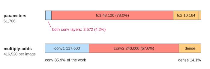
Count the work instead and the picture flips. Each conv weight is used at every output position: conv2's 2,416 weights do 240,000 multiply-adds per image. Each fc1 weight is used once. So the conv layers do 85.9% of the multiply-adds with 4.2% of the parameters (Demo 7: parameters vs multiply-adds). Parameters decide memory and how much data you need to train; multiply-adds decide speed.
The receptive field grows
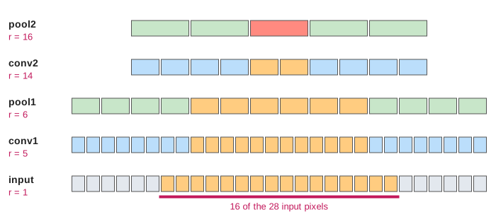
The receptive field of a value is the patch of input pixels it depends on. Two numbers track it, layer by layer: its size r and the jump j, the distance in input pixels between two neighbouring values. A layer with window K and stride S does
r ← r + (K − 1)·j j ← j·S
So r goes 1 → 5 (conv1) → 6 (pool1) → 14 (conv2) → 16 (pool2). The pools matter most: they double the jump, so conv2's 5×5 window covers 4 steps of 2 pixels, not 4 steps of 1. After flatten, every fc1 unit is wired to all 400 values and sees the whole digit (Demo 3: the receptive field grows).
For stacks of 3×3 layers with no pooling, and how attention reaches the whole image in one layer, see CNN vs Transformer.
Change one layer, watch the rest
A change early in the network ripples to every later shape and to the first dense layer:
| network | what changes | fc1 or head | total |
|---|---|---|---|
| LeNet-5 | — | 48,120 | 61,706 |
| no padding in conv1 | 28 → 24 → 12 → 8 → 4, flatten 256 | 30,840 | 44,426 |
| 32 filters in conv2 | conv2 4,832, flatten 800 | 96,120 | 112,122 |
| global average pooling | 5×5×16 → 16 → dense 10 | 170 | 2,742 |
Without padding, conv1 loses K − 1 = 4 pixels, and everything after it is smaller (Demo 4). Doubling the filters in conv2 only adds 2,416 conv weights, but it doubles flatten to 800 and fc1 to 96,120 (Demo 5). Global average pooling replaces each 5×5 map by its mean and drops fc1 and fc2: 2,742 parameters, 96% fewer (Demo 6). Modern CNNs such as ResNet end this way; see Transfer Learning for what happens to that head when a trained network is reused.
The original LeNet-5
LeCun et al. (1998) fed a 32×32 image to conv1 with no padding, which gives the same 28×28×6. Their subsampling layers averaged and had a trainable weight and bias per map, conv2 connected each map to only some of the 6 inputs, and the output used radial basis units. The tutorial version on this page keeps the shapes and swaps those details for max-pooling, full connections and softmax. The total is close: about 60,000 parameters.
What the page leaves out
The values flowing through the network and training it (see Neural Network: the Forward Pass and Backpropagation); activation functions, which add no parameters; batch normalization, which adds 2 parameters per channel; colour input (Cin = 3); dilation and groups in the conv formula; the effective receptive field, which is smaller than r because pixels near the edge of the patch count less; and memory for activations during training.
On the mind map
References
LeCun, Bottou, Bengio and Haffner: Gradient-based learning applied to document recognition (1998)
Dive into Deep Learning: Convolutional Neural Networks (LeNet)
Stanford CS231n notes: Convolutional Neural Networks
Araujo, Norris and Sim: Computing Receptive Fields of Convolutional Neural Networks (Distill, 2019)