Radix Tree Visualization

Compressing a trie

In a plain trie every letter is a node, so a word like DOG that shares nothing with the other words still costs a chain of three nodes, each with a single child. A radix tree (also called a compact prefix tree or, in its binary form, a Patricia trie) merges every such chain into one node that holds a whole string. A node is only needed where words branch or where a word ends.

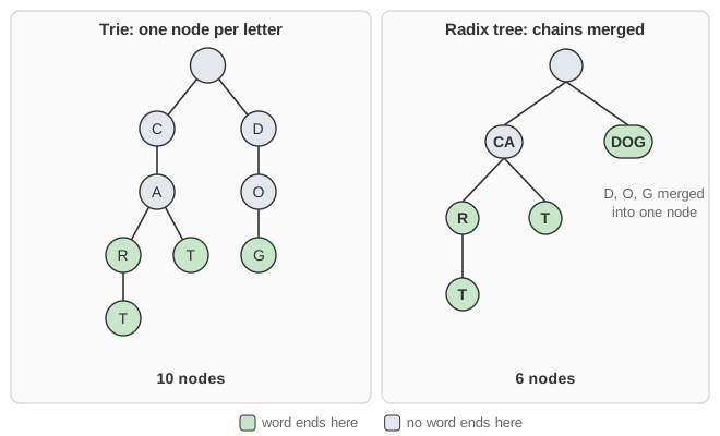
In the animation each circle shows the string (the label) stored at that node, and the edge into it is labelled with the first letter of that string. The word of a node is the concatenation of the labels on the path from the root. Green nodes are word ends; white nodes are only branching points. The tree keeps three rules:

1. the children of a node start with different letters, so the next letter of a word picks at most one child;
2. every node except the root has a non-empty label;
3. every white node has at least two children (a white node with one child is merged with it, and a white leaf is removed).

The page turns what you type into capital letters and drops everything that is not a letter (up to 12 letters).

Searching

Compare the word with the label of the current node, letter by letter (the animation highlights the pair being compared). Three things can happen: the word runs out or differs inside the label, and the word is not stored; the word ends exactly at the end of the label, and the answer is the node's colour; or the whole label matches and letters remain, and the search continues in the child that starts with the next letter.

find(node, s):                            // s = the part of the word not matched yet
    if node is null:
        return false
    k = length of the common prefix of s and node.label
    if k < length(node.label):            // s stops or differs inside this label
        return false
    if k == length(s):                    // s ends exactly at the end of the label
        return node.isWord
    return find(node.child[s[k]], s[k..]) // the rest of s starts with the letter s[k]

Inserting: splitting an edge

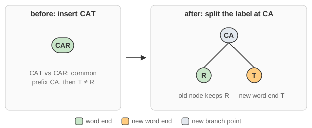
Insertion follows the same comparisons. The new case is a mismatch inside a label: the label has to be split at that point. A new white node takes the common part, the old node keeps the rest of its label and becomes its child, and the rest of the new word becomes a second, green child. If the new word ends exactly at the split point, the new node itself is green instead.

insert(node, s):                          // returns the subtree with s inserted
    if node is null:
        return new node(label = s, isWord = true)
    k = length of the common prefix of s and node.label
    if k == length(node.label):           // the whole label matches
        if k == length(s):
            node.isWord = true            // s ends here: turn it green
        else:
            c = s[k]
            node.child[c] = insert(node.child[c], s[k..])
        return node
    // mismatch at position k inside the label: split it
    top = new node(label = node.label[0..k-1], isWord = false)
    node.label = node.label[k..]
    top.child[node.label[0]] = node
    if k == length(s):
        top.isWord = true                 // s ends at the split point
    else:
        top.child[s[k]] = new node(label = s[k..], isWord = true)
    return top                            // replaces node in its parent

If the words have no common first letter, k = 0 and the split creates a node with an empty label. That is why the root is sometimes an empty circle.

Deleting: merging edges

Find the word and turn its node white. Then restore rule 3: a white node with no children leads to no word and is removed (which may leave its parent breaking the rule, so check the parent too); a white node with one child is merged with that child, whose label becomes the two labels joined together.

delete(word):
    node = the node where find(word) ends
    if node is null or not node.isWord:
        return                            // not stored: nothing to do
    node.isWord = false
    cleanup(node)

cleanup(node):
    if not node.isWord and node has no children:
        remove node from its parent       // or empty the tree
        cleanup(parent)                   // the parent may now break the rules
    else if not node.isWord and node has exactly one child c:
        c.label = node.label + c.label    // merge the two edges
        put c where node was              // c becomes the root if node was the root

A worked example

Insert CAR, CAT, CART, DOG and C into an empty tree (labels in quotes, * marks a green node):

insert CAR     insert CAT     insert CART      insert DOG           insert C
"CAR"*         "CA"           "CA"             ""                   ""
               +-"R"*         +-"R"*           +-"CA"               +-"C"*
               +-"T"*         |  +-"T"*        |  +-"R"*            |  +-"A"
                              +-"T"*           |  |  +-"T"*         |     +-"R"*
                                               |  +-"T"*            |     |  +-"T"*
                                               +-"DOG"*             |     +-"T"*
                                                                    +-"DOG"*

1. CAR: the tree is empty, so the whole word becomes one green node.
2. CAT: compared with CAR, the common prefix is CA and the third letter differs. The label is split: a new white node "CA" becomes the root, the old node keeps "R", and a new green node "T" holds the rest of CAT.
3. CART: the label "CA" matches completely, so the search goes on with RT in the R child. "R" matches too, and T is left over. There is no T child, so one is added.
4. DOG: not even the first letter matches "CA" (k = 0), so the split creates a white root with the empty label, with children "CA" and "DOG".
5. C: the empty root matches, and the search goes to the C child. The word ends after one letter of "CA", so "CA" is split into a green "C" with a white child "A".

Now find CA: "C" matches, then "A" matches and the word ends there, but "A" is white: not found. DO stops inside the label "DOG": not found. CARTS: after "T" the letter S is left and there is no S child: not found.

Delete CAR: "R" turns white and has one child, so it is merged with it into "RT"*. Delete CART: "RT" turns white and has no children, so it is removed; that leaves "A" white with one child, merged into "AT"*. Delete C: "C" turns white with one child and merges into "CAT"*. The tree is back to a white empty root with the children "CAT"* and "DOG"*.

Print lists the words in alphabetical order (children are visited from A to Z, and a node's word comes before the words below it). New random tree builds a tree from 10 to 50 random made-up words, listed below the tree in the order they are inserted.

Why it works

A radix tree is exactly the trie of the same words with every chain of white single-child nodes contracted into one edge. Splitting and merging only move the boundaries between labels; they never change which strings the paths spell. So every search follows the same letters it would follow in the trie and gives the same answer. Rule 1 makes the next child unique, and rule 3, restored after every deletion, keeps the tree as small as possible. As with a trie, the shape depends only on the set of words, not on the order of insertion.

Running time and space

For a word of length L, find, insert and delete compare each letter of the word at most once and visit at most L + 1 nodes: O(L) time, whatever the number of words n. A split or merge adds only constant work (plus copying a label). This is the same bound as a trie or a hash table (which needs O(L) to hash), and better than the O(L log n) of a balanced binary search tree of strings. Like a trie, and unlike a hash table, it also supports prefix queries and listing the words in order.

The gain over a trie is space. Every white node has at least two children, so there are fewer white nodes than green ones: at most 2n nodes in all, however long the words are, where a trie can need one node per letter. The letters themselves are stored once, in the labels.

Common mistakes and edge cases

• A word that ends inside a label (inserting C when the tree has "CA") still needs a split, with the upper part green. When searching, ending inside a label means "not found".
• A word that is a prefix of another (CAR and CART) is a green node with children: the word end is a flag, not "being a leaf".
• Deleting must restore the rules: remove a white leaf, then check its parent, which may now have a single child and need a merge. Forgetting the merge leaves a correct but no longer compressed tree.
• The root may have an empty label (when the words start with different letters), and after deletions a single child can become the new root.
• The empty string would be the root's flag. This page ignores empty input.

Variants and uses

The name comes from the radix r, the number of children a node may have: 26 for capital letters, 2 when the keys are taken bit by bit (a Patricia trie, which stores just the index of the next bit to test), or 256 for bytes. The adaptive radix tree (ART) picks the child array size per node and is used for indexes in in-memory databases.

Radix trees are used for IP routing, where the router needs the longest stored network prefix that matches the bits of a destination address; for URL routers in web frameworks, which match request paths such as /users/42 against the registered routes; in the Linux kernel (its radix tree, now the XArray) to find cached pages by index; and in key–value stores such as Redis. Like tries, they also serve autocomplete and dictionary lookups with less memory.

References

Radix tree