Topological Sort (DFS) Visualization

Topological sort with depth-first search

A topological order of a directed graph is a list of all its vertices such that for every edge u → v, u comes before v. Think of the edges as "must happen before" rules: course prerequisites, build steps, tasks in a project. A topological order is a schedule that respects every rule.

Such an order exists exactly when the graph has no directed cycle, i.e. it is a DAG (directed acyclic graph): on a cycle a → b → ... → a, vertex a would have to come before itself. The order is usually not unique.

The DFS method rests on one observation: when depth-first search finishes a vertex, everything that vertex must precede has already been finished. So if we list the vertices by decreasing finishing time (equivalently, put each vertex at the front of the list at the moment it finishes), we get a topological order.

Pseudocode

TopoSortDFS(G):
    order = empty list
    time = 1
    for each vertex u:  visited[u] = false
    for each vertex u:                    // restart so every vertex is covered
        if not visited[u]: DFS(u)
    return order

DFS(u):
    visited[u] = true;  d[u] = time++     // discovery time
    for each edge u -> v:
        if not visited[v]: DFS(v)
    f[u] = time++                         // finishing time
    insert u at the FRONT of order

Reading the animation

• The generated graphs are always DAGs: an edge is only ever created from a lower-numbered to a higher-numbered vertex, so the page never produces a cycle.
• The outer loop tries vertices 0, 1, 2, ..., and each vertex's neighbors are tried in increasing number (a row of the adjacency matrix).
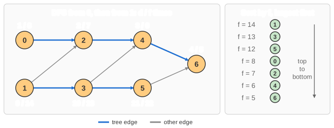
• The left panel is the call trace, one indented DFS(v) per call; a separator line marks a new DFS tree.
• Each vertex gets d = ... when discovered and f = ... when finished. Visited vertices are orange, the black circle is the vertex being explored, and tree edges turn blue.
• When a vertex finishes, a copy of its number flies into the Topological Order column and is inserted at the top, pushing the others down. When the animation ends, reading that column from top to bottom gives the answer.

Worked example

Seven vertices with edges (every edge goes from a lower to a higher number, like the page's graphs):

0 -> 2    1 -> 2    1 -> 3    2 -> 4
3 -> 4    3 -> 5    4 -> 6    5 -> 6

The DFS runs like this; the right column shows the Topological Order list after each finish:

DFS(0)             d[0] = 1
  DFS(2)           d[2] = 2
    DFS(4)         d[4] = 3
      DFS(6)       d[6] = 4
      finish 6     f[6] = 5     order: 6
    finish 4       f[4] = 6     order: 4 6
  finish 2         f[2] = 7     order: 2 4 6
finish 0           f[0] = 8     order: 0 2 4 6
---- vertex 1 is still unvisited: new DFS tree
DFS(1)             d[1] = 9
  1 -> 2: already visited
  DFS(3)           d[3] = 10
    3 -> 4: already visited
    DFS(5)         d[5] = 11
      5 -> 6: already visited
    finish 5       f[5] = 12    order: 5 0 2 4 6
  finish 3         f[3] = 13    order: 3 5 0 2 4 6
finish 1           f[1] = 14    order: 1 3 5 0 2 4 6

vertex :  0   1   2   3   4   5   6
d      :  1   9   2  10   3  11   4
f      :  8  14   7  13   6  12   5

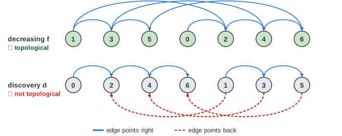
The result is 1, 3, 5, 0, 2, 4, 6, which is the list of vertices sorted by decreasing f. Check any edge, for example 3 → 4: f[3] = 13 > f[4] = 6, and 3 appears before 4. All eight edges pass this check. Note that the discovery order 0, 2, 4, 6, 1, 3, 5 is not topological: it puts 2 before 1 although there is an edge 1 → 2. (This trace was reproduced with the page's loops in Node, and the order was checked against every edge.)

Why finishing order works

It is enough to show: for every edge u → v of a DAG, f[v] < f[u]. Consider the moment DFS examines that edge, while u is still active (on the recursion stack). There are three possibilities for v:

1. v is unvisited: DFS calls DFS(v) right now, and that call returns before u's call does, so v finishes first. (Edge 0 → 2 above.)
2. v is visited and already finished: then f[v] is already set while u is not finished, so again f[v] < f[u]. (Edge 1 → 2 above: f[2] = 7 was set long before f[1] = 14.)
3. v is visited but not finished: then v is an ancestor of u on the recursion stack, so there is a path v → ... → u, and with the edge u → v this is a cycle. This is a back edge, which cannot happen in a DAG.

So every edge points from a later-finishing vertex to an earlier-finishing one, and listing by decreasing finishing time puts every u before its v. Case 3 also gives cycle detection: colour vertices white (unvisited), grey (active) and black (finished); if DFS ever meets a grey vertex, the graph has a cycle and no topological order exists. This page uses only a visited flag, which is enough because its graphs are always acyclic.

Running time and space

Each vertex is visited once and each edge examined once. With adjacency lists that is Θ(n + m) for n vertices and m edges; inserting at the front of a linked list (or pushing on a stack and reversing at the end) is O(1) per vertex. With an adjacency matrix, as in this animation, finding a vertex's neighbors scans a whole row, so the total is Θ(n²). Extra space is Θ(n): the flags, the times, the output list and the recursion stack, which can be n deep on a long path.

Common mistakes, edge cases and variants

• Forgetting to reverse. Appending vertices to the end of the list as they finish gives the order backwards (6, 4, 2, 0, 5, 3, 1 above), a reverse topological order.
• Using discovery order instead of finishing order: wrong, as the example shows.
• Only starting from vertex 0. Without the outer loop, vertices not reachable from the first start (1, 3 and 5 above) are missed.
• Cycles. On a graph with a cycle, the visited-flag version still outputs some list without complaining; it is just not a valid order. Use the three-colour check when the input might contain a cycle.
• Several valid answers. Changing the order in which vertices or neighbors are tried changes the result (starting the outer loop at vertex 1 instead of 0 gives 0, 1, 3, 5, 2, 4, 6 here). Any answer that satisfies every edge is correct.
• Deep recursion on huge graphs can overflow the call stack; an iterative DFS with an explicit stack avoids that.
• Kahn's algorithm (TopoSortIndegree.html) solves the same problem without recursion by repeatedly removing a vertex with no incoming edges, and reports a cycle naturally. The same finishing-time idea is also the first pass of Kosaraju's strongly connected components algorithm (ConnectedComponent.html).

Where it is used

• Build systems (make, compilers deciding which files to rebuild) and package managers installing dependencies before the packages that need them.
• Course planning with prerequisites, and scheduling jobs with precedence constraints.
• Spreadsheets recomputing cells after their inputs, and dataflow or task pipelines (workflow engines).
• Dynamic programming on DAGs: shortest and longest (critical) paths are computed in topological order in linear time.

References

Topological sorting

Depth-first search