Maximum flow
Think of a network of pipes: water enters at one vertex, leaves at another, and each pipe can carry only so much per second. How much can get through in total? The same question comes up for data in a computer network, goods on roads, or people assigned to jobs. This page computes the answer with the Ford-Fulkerson method, finding each augmenting path with a breadth-first search. That version is the Edmonds-Karp algorithm.
The problem: flow networks
A flow network is a directed graph G = (V, E) with a source s, a sink t, and a capacity c(u, v) ≥ 0 on every edge. A flow gives every edge a number f(u, v) with two rules:
- Capacity: 0 ≤ f(u, v) ≤ c(u, v) on every edge.
- Conservation: at every vertex other than s and t, the flow coming in equals the flow going out. Nothing is created or lost on the way.
The value of a flow, |f|, is the net flow out of the source: the flow on edges leaving s minus the flow on edges entering it. By conservation this equals the net flow into t. The maximum flow problem asks for a flow of the largest possible value.
In the animation every edge is labelled f/c: 3/7 means 3 units flow through an edge of capacity 7. The capacities are random numbers from 1 to 9.
Residual graphs and augmenting paths
A first idea is greedy: find any path from s to t whose edges are not full, push as much as the fullest edge allows, and repeat. That can get stuck below the maximum, because an early path may use an edge that a better solution would not use. The fix is to allow a later path to undo flow that was pushed earlier. The residual graph Gf records every way the current flow f can still change. For each edge u → v of the network it has up to two edges:
- a forward residual edge u → v with residual capacity c(u, v) − f(u, v), if that is positive: we can send that much more;
- a backward residual edge v → u with residual capacity f(u, v), if that is positive: we can cancel up to that much of the flow already on u → v.
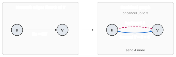
An augmenting path is a path from s to t in the residual graph. Its bottleneck is the smallest residual capacity along it. Augmenting by the bottleneck b adds b to the flow on every forward edge of the path and subtracts b from the flow on the real edge behind every backward edge. The capacity rule still holds (that is what the bottleneck guarantees). Conservation still holds too: each vertex inside the path gets one change on its way in and one on its way out, and they balance. The value of the flow grows by b.
If the network has both u → v and v → u (the random graphs here sometimes do), they are two separate edges, each with its own flow. The residual graph may then have two edges from u to v: the forward edge of u → v and the backward edge of v → u. The animation keeps them apart.
maxFlow(G, s, t):
    f(u, v) = 0 for every edge
    while there is a path P from s to t in the residual graph G_f:
        b = min residual capacity of the edges of P       // the bottleneck
        for each edge (u, v) of P:
            if (u, v) is a forward edge:   f(u, v) = f(u, v) + b
            else:                          f(v, u) = f(v, u) - b    // cancel flow
    return f                                             // |f| = total pushed

Edmonds-Karp: find P with a breadth-first search from s, so P has the fewest edges.

bfsPath(G_f, s, t):
    parent[v] = none for every v;  visited = {s};  queue = [s]
    while queue is not empty and t is not visited:
        u = dequeue()
        for each residual edge u → v with residual capacity > 0:
            if v is not visited:
                visited.add(v);  parent[v] = (u, forward or backward);  enqueue(v)
    return the path found by following parent from t back to s (or none)
Ford-Fulkerson is a method: it does not say how to find the path. Any search works (depth-first, widest path, ...). The Edmonds-Karp algorithm is the choice made here: a breadth-first search, which always finds a shortest augmenting path (fewest edges). That one choice gives a running time that does not depend on the capacities (see below).
How to read the animation
- Each iteration runs a BFS from the source in the residual graph. Visited vertices turn orange, the BFS tree edges turn green, and the queue is shown at the top left. The narration gives the residual capacity of every edge it looks at: c − f for a forward edge, f for a backward one.
- When the BFS reaches the sink, the augmenting path is drawn with forward edges in blue and backward edges in magenta, its bottleneck is found, and the flow on each of its edges is updated one by one. The table lists every path, its bottleneck, the edges whose flow it cancelled and the running total.
- When the BFS cannot reach the sink, the vertices it did reach are shaded blue: they form the source side of a minimum cut, and the cut edges are drawn in red.
Click a source vertex and then a sink vertex to run it, or type them and press Run Max Flow.
Worked example
Take the network with vertices s, a, b, c, d, e, t and these edges, every one with capacity 1:
s → a (1)    a → b (1)    b → t (1)
s → c (1)    c → b (1)
             a → d (1)    d → e (1)    e → t (1)
BFS looks at the neighbors of a vertex in alphabetical order.
Iteration 1.  BFS from s: visit a, c (from s); b, d (from a); c → b: b already visited;
              t (from b).  Shortest path s → a → b → t, residuals 1, 1, 1, bottleneck 1.
              Push 1:  f(s,a) = 1, f(a,b) = 1, f(b,t) = 1.            total flow 1

Iteration 2.  Residual graph: s → a, a → b and b → t are full; they now exist only
              as backward edges a → s, b → a and t → b.
              BFS from s: c (s → c, 1 − 0 = 1); b (c → b, 1 − 0 = 1);
              from b: b → t is full, but the backward edge b → a has residual
              f(a,b) = 1, so visit a; then d (a → d), e (d → e), t (e → t).
              Path s → c → b → a → d → e → t, where b → a is backward, bottleneck 1.
              Push 1:  f(s,c) = 1, f(c,b) = 1, f(a,b) = 1 − 1 = 0 (cancelled),
                       f(a,d) = 1, f(d,e) = 1, f(e,t) = 1.              total flow 2

Iteration 3.  BFS from s: s → a and s → c are both full and nothing enters s.
              Only s is reached, so there is no augmenting path.     maximum flow 2
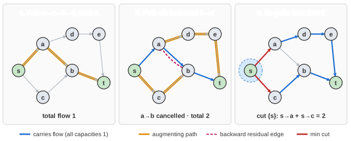
Look at what the backward edge did. After iteration 1 every real path from s to t has a full edge: s → c → b → t is blocked at b → t and everything through a is blocked at s → a. A greedy algorithm without backward edges would stop at 1. But the first path made a poor choice: the unit that reached a should go on to d, leaving b → t free for the unit coming from c. Cancelling the flow on a → b does exactly that re-routing: the final flow is s → a → d → e → t plus s → c → b → t, with nothing on a → b. Backward edges let the algorithm correct earlier decisions without searching over all of them.
At the end, the last BFS reached only S = {s}. The edges from S to the rest are s → a and s → c, with total capacity 2: the maximum flow.
Why it is correct: the max-flow min-cut theorem
A cut (S, T) splits the vertices into two sets with s ∈ S and t ∈ T. Its capacity c(S, T) is the total capacity of the edges from S to T (edges from T back to S do not count).
Every flow is at most every cut. All flow must cross from S to T somewhere. By conservation, |f| equals the flow on edges from S to T minus the flow on edges from T to S, which is at most c(S, T).
When the algorithm stops, some cut is met exactly. Let S be the vertices reachable from s in the final residual graph, and T the rest; t ∈ T because there is no augmenting path. Take an edge u → v with u ∈ S, v ∈ T. If it were not full, its forward residual edge would make v reachable, so it is full. Take an edge v → u from T into S. If it carried flow, its backward residual edge u → v would make v reachable, so it is empty. Then the formula above gives |f| = c(S, T).
Since no flow can be bigger than this cut, f is a maximum flow, and since no cut can be smaller than this flow, (S, T) is a minimum cut. This is the max-flow min-cut theorem: the following are equivalent, (1) f is a maximum flow, (2) the residual graph has no augmenting path, (3) |f| = c(S, T) for some cut. The final BFS gives the minimum cut for free, and the animation ends by showing it: the blue vertices are S and the red edges are the full edges leaving it.
Running time
With integer capacities, every augmentation raises the flow by at least 1, so the Ford-Fulkerson method stops after at most |f*| augmentations, where f* is a maximum flow. Each one costs O(E) to find a path and update it, for O(E · |f*|) in total. The flows it builds are integers at every step, so there is always an integer maximum flow (the integrality theorem).
That bound depends on the capacities, and a careless path choice really can be that slow. The classic example:
s → a (1000) s → b (1000) a → b (1) a → t (1000) b → t (1000)
Its maximum flow is 2000. A search that keeps choosing s → a → b → t and then s → b → a → t (using the backward edge of a → b) pushes only 1 unit each time and needs 2000 augmentations. With capacities of a million, a million times as many. With irrational capacities, a bad choice may never stop at all, and the flow may even converge to a value below the maximum.
Breadth-first search avoids this. BFS finds the two 2-edge paths first and is done after 2 augmentations. In general, the distance (in edges) from s to any vertex in the residual graph never decreases from one augmentation to the next. Each augmentation fills at least one edge of its path (the bottleneck edge), and before the same edge can be the bottleneck again, the distance to its start must grow by at least 2. So each of the E edges is the bottleneck at most about V/2 times, there are O(V · E) augmentations, and with O(E) per BFS the Edmonds-Karp algorithm runs in O(V · E2), whatever the capacities are.
Common mistakes
- Forgetting the backward edges. Without them the algorithm is the greedy one and can stop too early (1 instead of 2 in the worked example).
- Updating only one direction. Pushing b along u → v lowers its forward residual by b and raises the backward residual v → u by b. Code that keeps a residual matrix
r[u][v]must dor[u][v] -= b; r[v][u] += b. - Confusing capacity with residual capacity. The search and the bottleneck use c − f (or f for a backward edge), not c. A full edge is not in the residual graph at all.
- Antiparallel edges. With both u → v and v → u in the network, a single residual matrix still works if it starts with
r[u][v] = c(u, v)andr[v][u] = c(v, u), but the flow on each real edge can then no longer be read back directly. Keeping the flows per edge (as this page does) or adding a middle vertex on one of the two edges avoids the confusion. - Reading the min cut from the wrong graph. The source side is the set reachable in the final residual graph, not in the original network. And the cut capacity counts only edges from S to T.
Variants and faster algorithms
- Dinic's algorithm also uses shortest augmenting paths, but builds a BFS level graph once and then pushes a whole blocking flow through it with depth-first searches, before running BFS again. At most V phases, O(V2 · E) in total, and much faster in practice; O(E √V) on unit-capacity bipartite graphs.
- Push-relabel (Goldberg-Tarjan) works locally instead of along paths: vertices hold excess flow and push it to lower-labelled neighbors, raising their own label when stuck. O(V3) with FIFO order, O(V2 √E) with highest-label order; among the fastest in practice.
- Capacity scaling only uses paths whose bottleneck is at least Δ, halving Δ each round: O(E2 log C) for maximum capacity C.
- Bipartite matching as max flow. Add a source with an edge of capacity 1 to every left vertex, an edge of capacity 1 from every right vertex to a sink, and give each left-right edge capacity 1. An integer maximum flow picks each left and right vertex at most once, so its value is the size of a maximum matching. Ford-Fulkerson then runs in O(V · E); Hopcroft-Karp (Dinic on this network) in O(E √V).
- Minimum-cost flow adds a cost per unit on each edge and asks for the cheapest maximum flow (augment along cheapest residual paths, with backward edges costing the negative).
Applications
- Throughput of transport, pipeline, power and computer networks.
- Assignment problems through bipartite matching: workers to jobs, students to schools, flights to crews.
- Edge-disjoint and vertex-disjoint paths (Menger's theorem): with capacity 1 on every edge, the max flow is the number of disjoint routes, and the min cut the fewest links whose failure disconnects s from t.
- Image segmentation: pixels are vertices, and a minimum cut separates foreground from background at the cheapest boundary (graph cuts in computer vision).
- Project selection, open-pit mining and baseball elimination: choices with dependencies and profits become a minimum cut.
- Scheduling and circulations with demands, where each vertex must receive or send a given amount.