Strongly connected components (Kosaraju's algorithm)
Although the button says "Run Connected Component", the graphs on this page are directed, and what the animation computes are their strongly connected components (SCCs). Two vertices u and v are strongly connected if there is a path from u to v and a path from v back to u. This relation is an equivalence (every vertex reaches itself, and it is symmetric and transitive), so it splits the vertices into disjoint classes: the SCCs. Inside an SCC every vertex can reach every other; a vertex that lies on no cycle is an SCC on its own.
If you shrink every SCC to a single node you get the condensation of the graph, and the condensation is always a DAG (a cycle between two components would merge them into one). The method shown here is Kosaraju's algorithm (also credited to Sharir), which uses two depth-first searches. An alternative that needs only one DFS is shown on the Tarjan SCC page.
The idea
- Run a full DFS on G and record each vertex's finishing time
f(the moment its recursive call returns). - Build the transpose GT: the same vertices with every edge reversed. G and GT have exactly the same SCCs, because reversing every edge turns a path u → v into a path v → u.
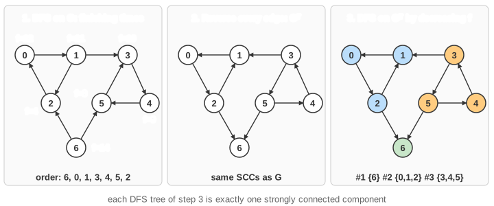
- Run DFS on GT, but in the outer loop try the vertices in decreasing finishing time from step 1. Every DFS tree built in this second pass is exactly one SCC.
Pseudocode
time = 1
DFS(G, u):
    visited[u] = true;  d[u] = time++
    for each edge u -> v in G:
        if not visited[v]: DFS(G, v)
    f[u] = time++                       // u is finished

Kosaraju(G):
    for each vertex u:  visited[u] = false
    for each vertex u:                  // pass 1: finishing times
        if not visited[u]: DFS(G, u)
    GT = transpose(G)                   // reverse every edge
    for each vertex u:  visited[u] = false
    k = 0
    for each vertex u in decreasing order of f[u]:   // pass 2
        if not visited[u]:
            k = k + 1
            DFS(GT, u)                  // every vertex reached here is in SCC #k
A common implementation avoids sorting: push u onto a stack when it finishes in pass 1, then pop vertices from that stack in pass 2.
Reading the animation
- Neighbors are tried in increasing vertex number (the code walks a row of the adjacency matrix), and the outer loop of pass 1 tries vertices 0, 1, 2, ...
- The text on the left is the call trace: each
DFS(v)line is indented under its caller, and a line is drawn where a new DFS tree starts. - Next to each vertex the labels
d = ...andf = ...show its discovery and finishing time (they also appear in the adjacency-list view). A visited vertex is filled orange, the black circle marks the vertex currently being explored, and edges used by the DFS (tree edges) turn blue. - After pass 1 the edges are redrawn reversed (the transpose; the adjacency list and matrix change too), a list
Vertex: v f = tappears and is sorted by decreasingf. Pass 2 then starts a new DFS from the first unvisited vertex of that list, and the left panel shows a headingCC #1,CC #2, ... with the vertices of each component in blue. Newd/fvalues are shown for pass 2, counted from 1 again.
Worked example
Take the directed graph with vertices 0 to 6 and edges
0 -> 1    1 -> 2    2 -> 0    1 -> 3
3 -> 4    4 -> 5    5 -> 3    6 -> 2    6 -> 5
By eye, the cycles 0 → 1 → 2 → 0 and 3 → 4 → 5 → 3 are components, and 6 is alone (nothing points back into it). Pass 1 on G, neighbors in increasing order:
DFS(0)            d[0] = 1
  DFS(1)          d[1] = 2
    DFS(2)        d[2] = 3
      2 -> 0: already visited
    finish 2      f[2] = 4
    DFS(3)        d[3] = 5
      DFS(4)      d[4] = 6
        DFS(5)    d[5] = 7
          5 -> 3: already visited
        finish 5  f[5] = 8
      finish 4    f[4] = 9
    finish 3      f[3] = 10
  finish 1        f[1] = 11
finish 0          f[0] = 12
---- vertices 1..5 are visited; 6 is not: new tree
DFS(6)            d[6] = 13
  6 -> 2, 6 -> 5: already visited
finish 6          f[6] = 14

vertex :  0   1   2   3   4   5   6
d      :  1   2   3   5   6   7  13
f      : 12  11   4  10   9   8  14
Sorted by decreasing f: 6 (14), 0 (12), 1 (11), 3 (10), 4 (9), 5 (8), 2 (4). The transpose has the edges 1→0, 2→1, 0→2, 3→1, 4→3, 5→4, 3→5, 2→6, 5→6. Pass 2 on GT:
CC #1   DFS(6)          6 has no outgoing edge in GT
        -> {6}
CC #2   DFS(0)          (next in the list: 0)
          DFS(2)        0 -> 2
            DFS(1)      2 -> 1   (1 -> 0: visited)
            2 -> 6: visited (already in CC #1)
        -> {0, 2, 1}
        1 is visited, skip
CC #3   DFS(3)
          3 -> 1: visited
          DFS(5)        3 -> 5
            DFS(4)      5 -> 4   (4 -> 3: visited)
            5 -> 6: visited
        -> {3, 5, 4}
        4, 5, 2 are visited, skip
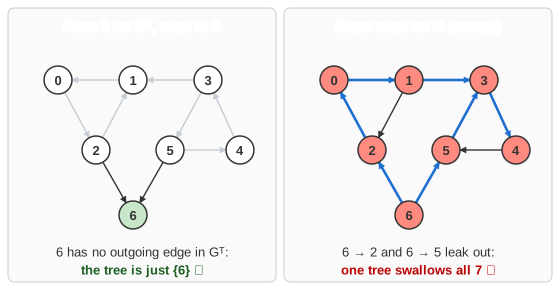
Result: three SCCs, {6}, {0, 1, 2} and {3, 4, 5}. Notice how the edges 2 → 6 and 3 → 1 in GT would have let a DFS "leak" into another component, but those components were already finished and marked visited. (This trace was checked by running the same loops as the page's code in Node.)
Why it works
Define f(C) for a component C as the largest finishing time of its vertices in pass 1. The key lemma:
If G has an edge from component C to a different component C', then f(C) > f(C').
Proof idea. Look at the first vertex x of C ∪ C' that pass 1 discovers. If x is in C, then at that moment every vertex of C and C' is unvisited and reachable from x, so all of them become descendants of x and finish before it: f(x) beats everything in C'. If x is in C', there is no path from C' back to C (otherwise they would be one component), so the whole of C' is finished before any vertex of C is even discovered. In the example: the edge 1 → 3 goes from {0,1,2} (f = 12) to {3,4,5} (f = 10), and 6 → 2 goes from {6} (f = 14) to {0,1,2}.
Now pass 2. It starts at the unvisited vertex r with the largest finishing time; let C be its component. C is strongly connected in GT as well, so DFS from r reaches all of C. Could it escape into another unvisited component C''? An edge C → C'' in GT is an edge C'' → C in G, so by the lemma f(C'') > f(C), which means C'' was started earlier in pass 2 and is already completely visited. So the tree rooted at r is exactly C, and by induction every later tree is exactly one component. Running pass 2 on G instead of GT would break this: from 6 the DFS would follow 6 → 2 and swallow everything.
A by-product: the components come out in topological order of the condensation of G (here {6}, then {0,1,2}, then {3,4,5}).
Running time and space
With n vertices and m edges stored as adjacency lists, each DFS visits every vertex once and every edge once, so it costs Θ(n + m). Building the transpose also takes Θ(n + m), and ordering by finishing time is free if you push vertices on a stack as they finish. Total: Θ(n + m) time, with Θ(n + m) extra space for GT plus Θ(n) for the flags, times and recursion stack.
With an adjacency matrix, finding the neighbors of a vertex means scanning a whole row, so each DFS costs Θ(n2); transposing the matrix is also Θ(n2). The animation works this way and additionally sorts the finishing times with insertion sort (O(n2)), which is fine for 8 or 18 vertices.
Common mistakes, edge cases and variants
- Wrong order in pass 2. It must be decreasing finishing time. Increasing order, or ordering by discovery time, can merge components.
- Wrong graph in pass 2. The second DFS must run on the transposed graph (equivalently: run pass 1 on GT and pass 2 on G).
- Unreached vertices. Both passes need the outer loop over all vertices; one DFS from vertex 0 does not see a vertex like 6 above that has no incoming path.
- Deep recursion. On large graphs (a path of a million vertices) the recursive DFS overflows the call stack; use an explicit stack.
- Undirected graphs. There, "connected components" need only one DFS or BFS per component (or a union-find structure); every edge works in both directions, so no transpose is needed.
- Tarjan's algorithm (TarjanSCC.html) finds the same components with a single DFS using low-link values and a stack, and does not need the transposed graph; it outputs components in reverse topological order. Both are linear time.
Where it is used
- 2-SAT: a formula is satisfiable exactly when no variable is in the same SCC as its negation in the implication graph.
- Condensing a graph to a DAG before running DAG algorithms (longest paths, dynamic programming, reachability queries).
- Finding groups of mutually recursive functions in compilers, circular imports between modules, and deadlock cycles in wait-for graphs.
- Analysing the structure of the web graph and social networks (the "giant strongly connected core").