The Bellman-Ford algorithm
Dijkstra's algorithm finds shortest paths quickly, but only when every edge weight is nonnegative. Once a vertex leaves its min-priority queue, Dijkstra's algorithm never looks at it again, and a negative edge found later could still lead to a cheaper path to that vertex. Negative weights come up naturally: think of a road trip where some legs earn you money, or of exchange rates, where taking logarithms turns "multiply the rates along a path" into "add the weights along a path."
The Bellman-Ford algorithm handles negative weights. It is slower than Dijkstra's algorithm, but it is simple, and it also tells you when there is no answer: when a negative cycle, a cycle whose weights add up to less than zero, is reachable from the source. Going around such a cycle again and again makes a path as cheap as you like, so the vertices it reaches have no shortest path at all.
Relaxing an edge
Like Dijkstra's algorithm, Bellman-Ford keeps for each vertex v a value dist[v], the weight of the best path from the source s to v found so far, and pred[v], the vertex just before v on that path. At the start, dist[s] is 0 and every other dist is ∞. To relax an edge (u, v) with weight w, ask whether going to u and then taking the edge beats the best path to v so far:
relax(u, v, w):
    if dist[u] + w < dist[v]:
        dist[v] = dist[u] + w
        pred[v] = u
In the animation, the Cost column holds dist and the Path column holds pred. A vertex is filled in once its cost is no longer ∞, that is, once some path to it has been found.
![Relaxing edge B to A with weight −3: before, dist[B] is 5 and dist[A] is 4 via S; since 5 − 3 = 2 is less than 4, after relaxing dist[A] is 2 and pred[A] is B](Images/bellmanford/relax.svg)
The algorithm
Dijkstra's algorithm is careful about the order in which it relaxes edges. Bellman-Ford isn't: it simply relaxes every edge, in any order, and repeats that n − 1 times, where n is the number of vertices. Then it makes one more pass to look for a negative cycle:
bellmanFord(s):
    for each vertex v:  dist[v] = ∞,  pred[v] = none
    dist[s] = 0
    repeat n − 1 times:
        for each edge (u, v) with weight w:
            relax(u, v, w)
    for each edge (u, v) with weight w:
        if dist[u] + w < dist[v]:
            report "negative cycle reachable from s"
If a whole pass lowers no cost, then no later pass can lower one either, since each pass sees the same costs as the one before it. So the algorithm can stop early, and it can skip the negative-cycle check too. The animation does both. On many graphs, only a few passes are needed.
Why n − 1 passes are enough
Suppose there is no negative cycle reachable from s. Then every vertex v that can be reached has a shortest path that is simple, one that visits no vertex twice, because cutting a cycle with nonnegative weight out of a path never makes it more expensive. A simple path visits at most n vertices, and so it has at most n − 1 edges.
Let the shortest path be s = v0, v1, …, vk = v. Pass 1 relaxes the edge (v0, v1), and after that dist[v1] is correct. Pass 2 relaxes (v1, v2), and after that dist[v2] is correct, and so on. It doesn't matter what else happens during a pass, because dist values only ever go down and never below the true shortest-path weight. After pass k, dist[v] is correct, and k ≤ n − 1.
So when there is no negative cycle, every cost is final after n − 1 passes and the extra pass can't lower anything. When a negative cycle is reachable, its costs can never all settle: adding up the relax test around the cycle would say its total weight is at least 0. So some edge on it can still be relaxed, and the extra pass finds it. Following pred back from that edge n times is sure to land on the cycle, and that is how the animation finds the cycle it colors red.
Running time
With n vertices and m edges, each pass relaxes m edges in Θ(m) time, and there are at most n passes, including the check. Bellman-Ford therefore runs in O(nm) time. That is slower than Dijkstra's algorithm with a binary heap, O(m lg n), so use Dijkstra's algorithm when all weights are nonnegative and Bellman-Ford when they might not be. If you need shortest paths between all pairs of vertices, see Floyd-Warshall.
Worked example
Vertices S, A, B, C and edges, relaxed in this order in every pass: A → C (2), B → A (−3), S → A (4), S → B (5). There are 4 vertices, so up to 3 passes.
start           S 0   A ∞   B ∞   C ∞
pass 1  A → C: A is ∞, skip      B → A: B is ∞, skip
        S → A: 0 + 4 = 4 < ∞     S → B: 0 + 5 = 5 < ∞      S 0   A 4   B 5   C ∞
pass 2  A → C: 4 + 2 = 6 < ∞     B → A: 5 − 3 = 2 < 4      S 0   A 2   B 5   C 6
pass 3  A → C: 2 + 2 = 4 < 6     (nothing else changes)    S 0   A 2   B 5   C 4
pass 4  nothing changes: no negative cycle
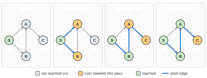
The shortest path to C, S → B → A → C (5 − 3 + 2 = 4), has 3 edges, so it needed 3 passes; with a luckier edge order it could have been found in one. Dijkstra's algorithm gets this graph wrong: it finalizes A at cost 4 before it looks at B, and never corrects it.
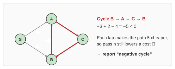
Add the edge C → B (−4). Now the cycle B → A → C → B costs −3 + 2 − 4 = −5, and the extra pass still finds an edge that lowers a cost, so the algorithm reports a negative cycle instead of distances.
Common mistakes
- Relaxing from an unreached vertex: skip edges whose start is ∞. With ∞ stored as a large number, "∞ + (−3)" looks like a real cost.
- Too few passes: n − 1 passes are needed in the worst case, because a shortest path can use n − 1 edges. Stopping early is only safe after a pass that changed nothing.
- Negative cycles that don't matter: the check only finds cycles reachable from the start. To detect any negative cycle in the graph, add a new vertex with a 0-cost edge to every vertex and start there.
- Undirected graphs: one negative undirected edge is already a negative cycle (u → v → u), so Bellman-Ford is used on directed graphs.
- SPFA (a queue of vertices whose cost just changed) is a common speed-up that has the same worst case.
Where the Bellman-Ford algorithm is used
Bellman-Ford is slower than Dijkstra's algorithm, and is chosen for what it can do that Dijkstra cannot: cope with negative edge weights, report that a negative cycle exists, and run in a distributed fashion where no single participant sees the whole graph.
- Distance-vector routing. RIP, and the distance-vector family in general, is a distributed Bellman-Ford: each router knows only its neighbours' tables, and repeatedly relaxes them. The algorithm's slow convergence is visible in the real protocol as the "count to infinity" problem, which is patched with split horizon and poison reverse.
- Currency arbitrage. Take the negative logarithm of each exchange rate and a profitable loop of trades becomes a negative cycle — precisely what Bellman-Ford detects. Trading systems use this to find and close such loops.
- Johnson's algorithm for all-pairs shortest paths runs Bellman-Ford once to compute a reweighting that removes negative edges, then runs Dijkstra from every vertex. On a sparse graph this beats Floyd-Warshall.
- Systems of difference constraints. Requirements of the form "x must start at least 3 units after y" form a graph whose shortest paths are a feasible schedule, and whose negative cycle is a proof that the constraints contradict each other. Used in scheduling and in compiler instruction scheduling.
- Graphs where costs can be gains: a discount, a refund, a reaction that releases energy. Any model where traversing an edge can reduce the total rules Dijkstra out.