A* search
Dijkstra's algorithm finds the shortest path from a start vertex to every vertex. It grows outward in rings of increasing distance, so to reach one particular goal it also explores everything that is closer to the start than the goal is, including places in the opposite direction. A* (pronounced "A-star") is Dijkstra's algorithm with a sense of direction: it uses an estimate of the remaining distance to the goal to explore promising vertices first.
g, h and f
For each vertex v, A* keeps three numbers:
g[v]: the cost of the best path from the start to v found so far. This is exactly Dijkstra'sdist.h[v]: the heuristic, an estimate of the cost from v to the goal. It is computed from v alone, without searching.f[v] = g[v] + h[v]: an estimate of the cost of the whole trip from the start to the goal through v.
![A winding blue path from S to v labelled g[v], the cost found so far, and a dashed straight line from v to G labelled h[v], the estimate; f[v] is their sum](Images/astar/g-h-f.svg)
A* keeps a set of open vertices, found but not yet expanded, which starts with only the start vertex. It repeatedly takes the open vertex with the smallest f, closes it, and relaxes its edges exactly as Dijkstra's algorithm does. It stops as soon as the goal is closed. With h = 0 everywhere, A* is Dijkstra's algorithm.
aStar(start, goal):
    g[start] = 0;  every other g = ∞
    open = {start}
    while open is not empty:
        u = the vertex in open with the smallest g[u] + h[u]
        move u from open to closed
        if u == goal:  return g[goal]      // follow Path back for the route
        for each edge (u, v) with cost w, v not closed:
            if g[u] + w < g[v]:
                g[v] = g[u] + w;  path[v] = u
                add v to open
    return "no path"
Choosing a heuristic
A* is guaranteed to return a shortest path when the heuristic is admissible: it never overestimates the true remaining cost. When it is also consistent, meaning h(u) ≤ w(u, v) + h(v) for every edge, a vertex's g is final once it is closed, just as in Dijkstra's algorithm. On maps, the straight-line distance to the goal is the classic choice: no road can be shorter than the straight line.
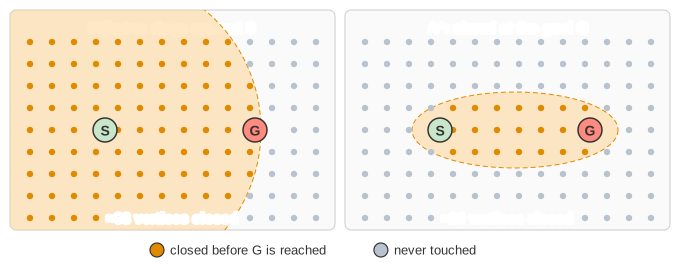
In this animation, each edge costs its drawn length divided by 20, rounded up, and h[v] is the straight-line distance from v to the goal divided by 20, rounded down. Rounding the costs up and the heuristic down keeps it both admissible and consistent. At the end, the page compares how many vertices A* closed with how many Dijkstra's algorithm would have closed before reaching the goal.
The better the estimate, the fewer vertices A* has to expand. A perfect heuristic would walk straight along a shortest path; h = 0 falls back to Dijkstra's algorithm. A heuristic that overestimates can make A* faster but may miss the shortest path.
Running time
In the worst case A* does everything Dijkstra's algorithm does, so with a binary heap for the open set it runs in O(m lg n) time for n vertices and m edges. In practice, with a good heuristic, it expands only a small part of the graph, which is why it is the standard choice for path finding in games, robotics and route planning. For a grid version, with walls, mud, heuristics and Jump Point Search, see Grid Pathfinding.
Worked example
Edges S–A (cost 1), A–G (10), S–B (4) and B–G (2), with heuristic h(S) = 5, h(A) = 4, h(B) = 2, h(G) = 0. It is admissible: the true costs to G are 6, 10, 2 and 0.
open {S: g 0, f 0+5 = 5}
expand S (f 5):  A: g 1, f 1+4 = 5    B: g 4, f 4+2 = 6
expand A (f 5):  G: g 1+10 = 11, f 11            open: B f 6, G f 11
expand B (f 6):  G: g 4+2 = 6 < 11, so g = 6, f 6, path[G] = B
expand G (f 6):  G is closed: stop.  Shortest path S → B → G, cost 6
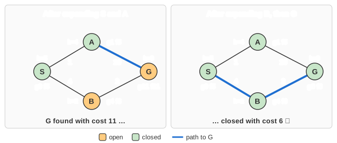
Notice that G was found with cost 11 long before it was closed with cost 6. Stopping as soon as the goal is discovered would have returned the wrong path; A* must stop when the goal has the smallest f of all open vertices.
Common mistakes
- Stopping when the goal is first discovered instead of when it is closed (see the example).
- An overestimating heuristic, for example straight-line distance on a map where some roads are faster than "distance / top speed" suggests, can return a longer path.
- An admissible but inconsistent heuristic is still optimal only if closed vertices may be reopened when a cheaper path to them turns up. With a consistent heuristic, as on this page, that never happens.
- Ties in f: preferring the vertex with the smaller h (closer to the goal) usually expands fewer vertices; this page does that.
- On grids, the heuristic must match the allowed moves: Manhattan distance for 4-way moves, octile or Chebyshev distance when diagonals are allowed.
Where A* is used
A* is Dijkstra's algorithm with a sense of direction: the heuristic biases the search towards the goal instead of spreading evenly in all directions. Where Dijkstra explores a circle around the start, A* explores an ellipse aimed at the target, and on a large map that is the difference between practical and not.
- Game pathfinding. This is the canonical use and it is close to universal: characters moving over a grid, a navigation mesh or a waypoint graph. Almost every game engine ships an A* implementation, usually with Manhattan or Euclidean distance as the heuristic.
- Robotics. Motion planning over an occupancy grid, and the incremental variants D* and D* Lite that repair the existing path when the robot discovers the map was wrong, rather than replanning from scratch.
- Route planning. On road networks, straight-line distance is a weak heuristic; real systems use landmark-based bounds (the ALT method), which are far more informative and keep the search narrow across an entire continent.
- Puzzle solving and planning. The 15-puzzle with a Manhattan distance heuristic is the textbook case; automated planners in AI use the same framework with heuristics derived automatically from a relaxed version of the problem.
- Sequence and decoding problems. Beam search and stack decoders in speech recognition and machine translation score partial hypotheses with the same cost-so-far plus estimated-cost-to-go idea.
Everything depends on the heuristic being admissible — never an overestimate of the true remaining cost. Overestimate and A* still returns a path, quickly, but no longer necessarily the shortest one; some systems accept that trade deliberately. With h = 0 the heuristic tells you nothing and A* degenerates into exactly Dijkstra's algorithm.