Dijkstra vs A*
This page builds one random graph, draws it twice, and runs Dijkstra's algorithm in the left copy and A* in the right copy at the same time, one expansion at a time. Both are looking for a shortest path between the same two vertices, on the same edges, with the same costs. The only thing that differs is which vertex each one picks next — and after a handful of steps the two pictures no longer look anything alike.
One loop, two priorities
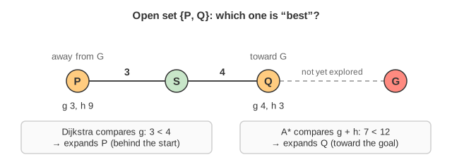
Both algorithms are the same loop. Keep a set of open (discovered but not yet expanded) vertices; repeatedly take the best one out, mark it closed, and relax its edges. The single difference is the word "best":
bestFirstSearch(start, goal):
    g[start] = 0;  every other g = ∞
    open = {start}
    while open is not empty:
        u = the vertex in open minimizing  f(u)        <-- THE ONLY DIFFERENCE
                Dijkstra:  f(u) = g[u]
                A*:        f(u) = g[u] + h[u]
        move u from open to closed
        if u == goal:  return g[goal]
        for each edge (u, v) with cost w, v not closed:
            if g[u] + w < g[v]:
                g[v] = g[u] + w;  path[v] = u
                add v to open
    return "no path"
So A* with h = 0 everywhere is Dijkstra's algorithm. On this page the left panel really is running the right panel's code with the heuristic switched off — one Search object, constructed twice.
A circle and a cigar
Dijkstra always expands the open vertex closest to the start, so the closed set grows as a ball of radius g around the start, in every direction equally. To reach a goal at distance 40 it must first close every vertex within 40 of the start — including everything directly away from the goal.
A* adds h, the straight-line distance still to go. Closing a vertex now requires g + h to be small, which means the vertex must be both cheap to reach and pointing at the goal. Vertices behind the start have a large h and sink to the bottom of the queue. The closed set stretches into an ellipse — a cigar — with the start and the goal at its ends. The tighter the heuristic, the thinner the cigar; a perfect heuristic would walk straight down a shortest path.
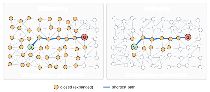
Watch the vertex labels to see this directly. The left panel labels each vertex with its g; the right panel labels an undiscovered vertex with its h (gray) and a discovered one with its f = g + h (black). The gray h numbers are the map A* is steering by before it has walked anywhere.
The heuristic on this page
Vertices are scattered on a jittered grid, and an edge between two of them costs ⌈straight-line length / 20⌉. The heuristic is h(v) = ⌊straight-line distance from v to the goal / 20⌋.
Rounding the costs up and the heuristic down is what makes this safe. It keeps h admissible — never more than the true remaining cost, since no route can be shorter than the straight line — and consistent: h(u) ≤ w(u, v) + h(v) for every edge. Consistency is the stronger property, and it is the one that matters: with it, a vertex's g is final the moment it is closed, exactly as in Dijkstra's algorithm, so no vertex is ever reopened and A* is guaranteed to return a shortest path. That is why the two panels always finish with the same cost, however different their pictures look.
What "in parallel" means here
The two searches are stepped in lockstep: at step k, each side has expanded k vertices. Expansions — not milliseconds — are the honest unit of comparison, because an expansion costs each algorithm the same thing: one queue removal plus one pass over the vertex's edges. The bar of ticks under each panel counts them, and it is the whole scoreboard: A* wins when its bar stops sooner.
Timing the two with a stopwatch on a twenty-vertex graph would mostly measure the priority queue, the JIT and the browser. Counting expansions measures the algorithms.
When A* does not help
- No usable geometry. A* needs a lower bound on the remaining cost that it can compute without searching. On a road map, straight-line distance is free. On a social graph, a dependency graph or a state machine, there is often nothing better than
h = 0— and then A* is Dijkstra with extra bookkeeping. - The goal is nearby. If the goal is two hops away, Dijkstra barely explores anything and there is nothing to save.
- Plateaus. When many routes tie on
f— common on uniform grids — A* has to sweep the whole tied region, and a weak heuristic degenerates toward Dijkstra. Breaking ties toward the smallerh(this page does) helps. - You want every distance. Dijkstra solves one-to-all. A* solves one-to-one. If you need the distance to every vertex, the heuristic has nothing to aim at and Dijkstra is the right algorithm.
- The heuristic itself costs something. A cheap, slightly worse
hoften beats an expensive, sharper one.
Worked example
Edges S–A (cost 1), A–G (10), S–B (4), B–G (2); heuristics h(S) = 5, h(A) = 4, h(B) = 2, h(G) = 0 (admissible: the true costs to G are 6, 10, 2, 0).
                 Dijkstra (f = g)                 A* (f = g + h)
expansion 1      S  (g 0)                         S  (f 0+5 = 5)
expansion 2      A  (g 1)                         A  (f 1+4 = 5)
expansion 3      B  (g 4)                         B  (f 4+2 = 6)
expansion 4      G  (g 6)  -> stop                G  (f 6+0 = 6)  -> stop

Same path S -> B -> G, cost 6, and on this tiny graph the same four expansions:
with only four vertices there is nothing for the heuristic to skip.
That last line is worth taking seriously: A* is never worse than Dijkstra in expansions (with a consistent heuristic), but on a small or badly-shaped graph it is often merely equal. Press New Random Graph a few times on this page and you will see the margin swing from "barely any" to "half the graph".
Common mistakes
- Stopping when the goal is first discovered instead of when it is closed. The goal is often found on an expensive path long before its cheapest one turns up. See the worked example on the A* page, where G is discovered with cost 11 and closed with cost 6.
- An overestimating heuristic. It makes A* faster and can make it wrong: the search commits to a route and closes the goal before the cheaper one is examined.
- Comparing wall-clock time on a toy graph. Count expansions.
- Assuming A* always wins. It wins when the heuristic is informative and the goal is far. Otherwise the two panels finish neck and neck.
- A heuristic that does not match the allowed moves. On a grid: Manhattan distance for 4-way movement, octile or Chebyshev when diagonals are allowed. Straight-line distance is admissible for both, but looser, so it explores more.