Strongly connected components
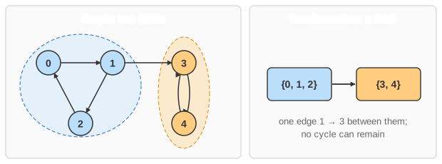
In a directed graph, vertex u can reach vertex v when there is a path from u to v. Two vertices are strongly connected when each can reach the other. That relation splits the vertices into groups called strongly connected components (SCCs): inside a component every vertex can reach every other, and no larger set has that property. A vertex that lies on no cycle forms a component by itself.
If you shrink each component to a single vertex, the result is always a directed acyclic graph (the condensation). That makes SCCs a common first step: compilers use them to find mutually recursive functions, package managers to find circular dependencies, and 2-SAT solvers to decide satisfiability.
Tarjan's idea
Robert Tarjan's algorithm finds every component in a single depth-first search. (The Connected Components page shows Kosaraju's approach, which needs two searches and the transposed graph.) The search gives each vertex two numbers:
index[v]: the order in which the search first reaches v (0, 1, 2, …).low[v]: the smallest index reachable from v by going down the DFS tree and then taking at most one edge back to a vertex that is still on the stack.
Every visited vertex is pushed on a stack and stays there until its component is complete. When the search finishes a vertex u and finds low[u] == index[u], nothing below u reaches anywhere above it, so u is the first vertex of its component that the search reached, its root. The vertices on the stack from the top down to u are exactly that component, and they are popped off together.
strongConnect(u):
    index[u] = low[u] = counter++
    push u;  onStack[u] = true
    for each edge u → v:
        if v has no index:              // tree edge
            strongConnect(v)
            low[u] = min(low[u], low[v])
        else if onStack[v]:             // edge back into the current search
            low[u] = min(low[u], index[v])
        // else: v is in a finished component; ignore the edge
    if low[u] == index[u]:              // u is a component's root
        pop vertices down to u; they form one SCC

for each vertex v with no index:  strongConnect(v)
Why ignore an edge to a vertex that is no longer on the stack? That vertex already belongs to a finished component. If it could reach back to u, it would have been part of u's component and would still be on the stack. So the edge can't help u reach anything above it.
In the animation, the table shows index, low and whether each vertex is on the stack, and the stack is drawn next to it. Tree edges turn blue, a vertex turns orange when the search reaches it, and each finished component gets its own color.
Running time
Each vertex is visited once, pushed once and popped once, and each edge is examined once. Tarjan's algorithm therefore runs in Θ(n + m) time for n vertices and m edges, the same as a plain depth-first search. As a bonus, components are found in reverse topological order of the condensation: a component is always completed before any component that has an edge into it.
Worked example
Take the edges 0 → 1, 1 → 2, 2 → 0, 1 → 3, 3 → 4 and 4 → 3. Start the search at 0:
visit 0            index = low = 0          stack: 0
visit 1 (0 → 1)    index = low = 1          stack: 0 1
visit 2 (1 → 2)    index = low = 2          stack: 0 1 2
  2 → 0: 0 is on the stack      low[2] = min(2, index[0]) = 0
  2 done: low 0 ≠ index 2, so 2 stays on the stack
back at 1          low[1] = min(1, low[2]) = 0
visit 3 (1 → 3)    index = low = 3          stack: 0 1 2 3
visit 4 (3 → 4)    index = low = 4          stack: 0 1 2 3 4
  4 → 3: 3 is on the stack      low[4] = min(4, index[3]) = 3
  4 done: low 3 ≠ index 4, stays
back at 3          low[3] = min(3, low[4]) = 3
  3 done: low 3 = index 3 → pop down to 3:   SCC {3, 4}      stack: 0 1 2
1 done: low 0 ≠ index 1, stays
0 done: low 0 = index 0 → pop down to 0:     SCC {0, 1, 2}   stack: empty
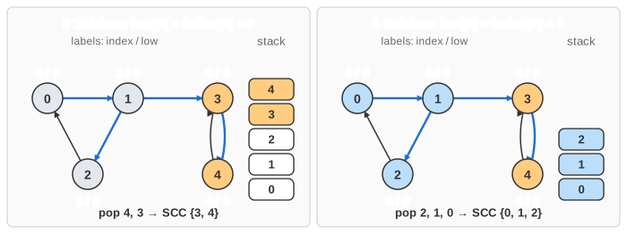
The component {3, 4} is found first even though the search reached it later: there is an edge from {0, 1, 2} into {3, 4}, and components always come out in reverse topological order.
Common mistakes
- Forgetting the on-stack test. An edge to a vertex of an already finished component must be ignored. Using its index would lower
lowand wrongly glue two components together. - Popping too little or too much: pop until u itself has been popped, not until the stack is empty.
- Recursion depth: a path of 100,000 vertices overflows the call stack in most languages; production code uses an explicit stack.
- Using
low[v]instead ofindex[v]for an edge to an on-stack vertex also finds the right components, but the textbook version, and the proofs, useindex[v].
Where strongly connected components are used
Condensing each strongly connected component to a single vertex turns any directed graph into a directed acyclic graph. That is the move behind most applications: cycles are what make a directed graph hard to reason about, and finding them in one linear pass lets everything downstream assume there are none.
- Compilers. Mutually recursive functions form an SCC of the call graph. Condensing it yields the order in which groups of functions can be analysed, type-checked or optimised — and each SCC must be handled as a unit, because none of its members can be understood alone.
- 2-SAT. Build the implication graph of a 2-CNF formula; it is satisfiable exactly when no variable lies in the same SCC as its own negation, and the condensation gives the assignment. This solves 2-SAT in linear time, and it is the standard method.
- Dependency analysis. Circular dependencies between packages, modules, microservices or database tables are SCCs. A build tool that reports "circular import" has just run one of these algorithms.
- Deadlock detection. A cycle in a wait-for graph of processes and resources is a deadlock; the SCC is exactly the set of processes involved.
- Model checking and dataflow analysis, where a loop in the state graph must be found and reasoned about before a fixed-point computation can be run.
- Link analysis. The classic "bowtie" description of the web — a large strongly connected core, with pages leading in and pages leading out — comes from this decomposition, and PageRank-style computations use the condensation to handle each part appropriately.
Tarjan's algorithm does it in one depth-first pass; Kosaraju's takes two passes and is easier to remember; both are O(n + m).