The idea: probability is area under a curve
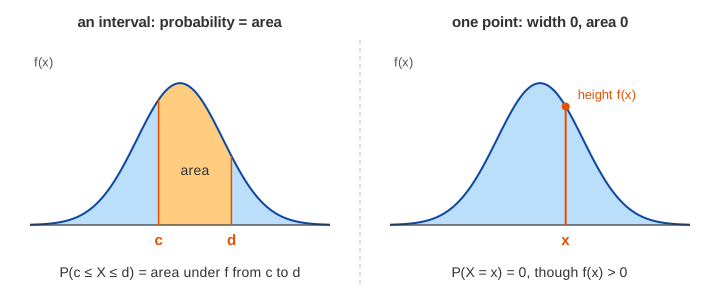
A continuous random variable X can take any value in a range: a height, a waiting time, a proportion. There are too many values to give each one its own probability. So X is described by a curve, its density f(x). The curve is tall where values are common and low where they are rare. The chance that X lands between c and d is the area under the curve from c to d. The whole area is 1.
The canvas draws one density at a time. Pick a distribution, its parameters and an interval [c, d]. The page shades the area over the interval in orange and prints P(c ≤ X ≤ d). The purple line is the mean and the purple bar reaches one standard deviation σ to each side. The card on the right shows the formulas with the current numbers. Demo: uniform, probability is area is the simplest case.
A density is not a probability
The height f(x) is probability per unit of x. It is not the chance of x. For any single value, P(X = x) = 0. Shrink the interval around a point and the area shrinks with it: for the standard normal the areas around 0 are 0.6827, 0.3829, 0.0797, 0.0080 and then 0, while the height stays f(0) = 0.3989 (Demo: one point has probability 0). This is why P(c ≤ X ≤ d) and P(c < X < d) are the same number.
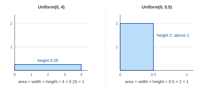
Because a height is not a probability, it can be above 1. Uniform(0, 0.5) has height 2 everywhere. Its area is still 0.5 × 2 = 1 (Demo: a height above 1). Only two rules hold for every density: f(x) ≥ 0, and the total area is 1.
Uniform(a, b): equally likely anywhere
X is as likely to land in one part of [a, b] as in any other part of the same width. The density is flat.
f(x) = 1/(b − a)   for a ≤ x ≤ b
mean (a + b)/2     variance (b − a)²/12
Every area is a rectangle. For Uniform(0, 4) the height is 0.25, so P(1 ≤ X ≤ 3) = 2 × 0.25 = 0.5, and P(0 ≤ X ≤ 2) is 0.5 too: same width, same chance. The mean is 2 and the variance is 16/12 = 1.3333 (Demo: uniform, probability is area).
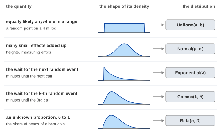
Normal(μ, σ): many small effects added up
Add up many small independent effects and the total follows the bell curve. Heights, measuring errors and test scores are close to it.
f(x) = e^(−(x − μ)²/(2σ²)) / (σ√(2π))
mean μ             variance σ²
For Normal(0, 1), P(−1 ≤ X ≤ 1) = 0.6827 and P(−2 ≤ X ≤ 2) = 0.9545: about 68% of the area is within one σ of the mean and about 95% within two (Demo: normal, 68% and 95%). The two parameters do different jobs. μ slides the bell along the axis. σ widens it, and a wider bell must be lower, because the area stays 1: the peak 1/(σ√(2π)) falls from 0.3989 at σ = 1 to 0.1995 at σ = 2 (Demo: normal, μ slides and σ widens). More on the normal distribution and z-scores page.
Exponential(λ): the wait for the next event
Events come at random at a rate of λ per unit of time: calls, buses, clicks. X is the wait until the next one.
f(x) = λ·e^(−λx)   for x ≥ 0
mean 1/λ           variance 1/λ²
The curve is tallest at 0 and only falls: short waits are the most likely. With λ = 1, P(X ≤ 1) = 1 − e−1 = 0.6321, and the mean and the variance are both 1. A larger λ means events come faster, so the curve starts higher and drops faster: with λ = 2 it starts at 2 and P(X ≤ 1) = 0.8647 (Demo: exponential, the wait for the next event). See exponential waiting times for the memoryless property.
Gamma(k, θ): the wait for the k-th event
Now wait for the k-th event, not the first. Each single wait has mean θ (so θ = 1/λ), and X is the sum of k of them. The page uses whole numbers for k.
f(x) = x^(k−1)·e^(−x/θ) / (θ^k·(k − 1)!)   for x ≥ 0
mean kθ            variance kθ²
With k = 1 this is the exponential. As k rises the peak moves right, to (k − 1)θ, and the curve looks more like a bell. Gamma(3, 1) is the sum of 3 exponential waits: mean 3, variance 3, and P(X ≤ 3) = 0.5768 (Demo: gamma, the wait for the k-th event).
Beta(α, β): an unknown proportion
X is a proportion between 0 and 1 that we are not sure of: the share of heads of a bent coin, a click rate. The page uses whole numbers for α and β.
f(x) = x^(α−1)·(1 − x)^(β−1) / B(α, β)   for 0 ≤ x ≤ 1
B(α, β) = (α − 1)!·(β − 1)! / (α + β − 1)!
mean α/(α + β)     variance αβ / ((α + β)²(α + β + 1))
Beta(1, 1) is flat: the uniform on [0, 1]. A larger β pushes the curve toward 0 and a larger α pushes it toward 1. Beta(2, 5) has mean 2/7 = 0.2857 and variance 0.0255, and P(X ≤ 0.5) = 0.8906 (Demo: beta, an unknown proportion). One way to read it: after seeing α − 1 successes and β − 1 failures, starting from "no idea", this curve is what we believe about the proportion. That is the prior and posterior on the frequentist vs Bayesian page.
All five side by side
| distribution | x can be | density f(x) | mean | variance | typical use |
|---|---|---|---|---|---|
| Uniform(a, b) | a to b | 1/(b − a) | (a + b)/2 | (b − a)²/12 | a random point in a range, rounding error |
| Normal(μ, σ) | any number | e−(x−μ)²/(2σ²) / (σ√(2π)) | μ | σ² | sums and averages, measuring error |
| Exponential(λ) | 0 and up | λe−λx | 1/λ | 1/λ² | wait for the next event |
| Gamma(k, θ) | 0 and up | xk−1e−x/θ / (θk(k − 1)!) | kθ | kθ² | wait for the k-th event |
| Beta(α, β) | 0 to 1 | xα−1(1 − x)β−1 / B(α, β) | α/(α + β) | αβ / ((α + β)²(α + β + 1)) | an unknown proportion |
How they relate
- Exponential = Gamma with k = 1. The wait for the first event is the simplest gamma. With rate λ, θ = 1/λ.
- Gamma(k, θ) = a sum of k exponential waits. That is how the page draws its gamma samples.
- Beta(1, 1) = Uniform(0, 1). Knowing nothing about a proportion is the flat curve.
- Sums of many things → normal. Gamma with a large k is already close to a bell. The central limit theorem says why.
Samples and the histogram
A sample is one random value of X. Draw many, count how many fall in each bin and divide by the number of samples and by the bin width. The bars then sit on the same scale as the density. With 10 samples they are rough. With 200 they are close to the curve, and the share of samples inside [c, d] is close to the area: for Normal(0, 1) and [−1, 1] it comes near 0.68 (Demo: 200 samples pile up into the curve). So the area is also a long-run share: draw X again and again, and that part of the draws lands in the interval. The samples come from a fixed seed, so the same clicks always give the same bars.
See also PDF vs CDF for the running total of the area, and discrete distributions for variables that are counted, not measured.
What the page leaves out
- The CDF in detail: its curve, quantiles and the median. The page only uses it to compute the areas.
- Other common curves: chi-square, Student's t, log-normal, Weibull, Cauchy.
- Gamma and beta with parameters that are not whole numbers, where (k − 1)! becomes the gamma function Γ(k).
- Discrete distributions such as the binomial and the Poisson, where single values do have probabilities.
- Two or more variables at once: joint densities, independence and correlation.
- Fitting a distribution to real data.