The idea: a list of chances that add up to 1
A discrete random variable X takes whole-number values: the number of heads, the number of flips, the face of a die. Its probability mass function (PMF) gives one number for each value k: P(X = k), the chance that X is exactly k. Every P(X = k) is between 0 and 1, and all of them together add up to 1, because X must take some value.
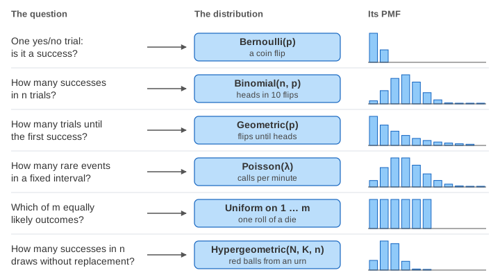
The page shows six common PMFs. Each one answers a different question about a simple experiment. The top strip shows the experiment. The chart draws one bar per value k. The card lists the formula, the mean E[X] (the long-run average of X) and the variance Var(X) (how far X spreads around the mean). The square root of the variance is the standard deviation σ. On the chart the red line is the mean and the yellow band is mean ± σ.
Bernoulli: one yes/no trial
One trial that succeeds with probability p. X = 1 for a success and 0 for a failure.
P(X = 1) = p        P(X = 0) = 1 − p
E[X] = p            Var(X) = p(1 − p)
With p = 0.3 the two bars are 0.7 and 0.3, the mean is 0.3 and the variance is 0.3 × 0.7 = 0.21 (Demo: Bernoulli, one yes/no trial). The variance is largest at p = 0.5, where the outcome is the hardest to guess.
Binomial: successes in n trials
Repeat the same Bernoulli trial n times, each one independent of the others, and count the successes. There are C(n, k) ways to place k successes among n trials, and each way has chance pk(1 − p)n−k.
P(X = k) = C(n, k) · p^k · (1 − p)^(n − k),   k = 0 … n
E[X] = np           Var(X) = np(1 − p)
For n = 10 and p = 0.3: P(X = 3) = 120 × 0.3³ × 0.7⁷ = 0.2668, the mean is 3 and the variance is 2.1 (Demo: binomial, successes in 10 trials). At p = 0.5 the bars are symmetric and P(X = 5) = 0.2461. At p = 0.1 they pile up on the left with a tail to the right (Demo: binomial shape, p = 0.5 then p = 0.1). The numbers C(n, k) are the rows of Pascal's triangle.
Geometric: trials until the first success
Keep repeating the trial until the first success. X is the number of trials, counting the successful one. To get X = k you need k − 1 failures and then a success.
P(X = k) = (1 − p)^(k − 1) · p,   k = 1, 2, 3, …
E[X] = 1/p          Var(X) = (1 − p)/p²
With p = 0.3: P(X = 1) = 0.3, P(X = 3) = 0.7² × 0.3 = 0.147, the mean is 1/0.3 = 3.33 and the variance is 0.7/0.09 = 7.78 (Demo: geometric, trials until the first success). The tallest bar is always k = 1, and each next bar is 1 − p times the one before. X has no upper limit, so the chart stops at k = 12 and says how much probability lies beyond.
Poisson: rare events in a fixed interval
Events happen at random moments, independent of each other, at an average rate of λ per interval: calls per minute, typos per page. X is the number of events in one interval.
P(X = k) = e^(−λ) · λ^k / k!,   k = 0, 1, 2, …
E[X] = λ            Var(X) = λ
With λ = 3: P(X = 3) = e⁻³ × 27 / 6 = 0.2240. The mean and the variance are both 3 (Demo: Poisson, rare events in an interval). "Mean equals variance" is a quick test of whether count data look Poisson.
Discrete uniform: equally likely outcomes
Every outcome has the same chance. A fair die has 6 faces, so each bar is 1/6 = 0.1667.
P(X = k) = 1/m,   k = 1 … m          (a die: m = 6)
E[X] = (m + 1)/2    Var(X) = (m² − 1)/12
For the die the mean is 3.5 and the variance is 35/12 = 2.92 (Demo: fair die, all outcomes equal). The mean 3.5 is not a face of the die. A mean does not have to be a possible outcome.
Hypergeometric: draws without replacement
An urn holds N balls and K of them are red. Draw n balls and do not put any back. X is the number of red balls drawn. Count the ways: choose k of the K red balls and n − k of the N − K others, out of all C(N, n) ways to draw n balls.
P(X = k) = C(K, k) · C(N − K, n − k) / C(N, n)
E[X] = n·K/N        Var(X) = n · (K/N)(1 − K/N) · (N − n)/(N − 1)
With N = 20, K = 6, n = 5 the mean is 5 × 6/20 = 1.5 and the variance is 0.83. Binomial(5, 0.3) is the same draw with replacement. It has the same mean 1.5 but a larger variance, 1.05 (Demo: hypergeometric vs binomial). Without replacement each red ball drawn leaves fewer red balls behind, which pulls the count back toward the mean.
All six side by side
| Distribution | Values k | P(X = k) | Mean | Variance | Typical use |
|---|---|---|---|---|---|
| Bernoulli(p) | 0, 1 | p for 1, 1 − p for 0 | p | p(1 − p) | one click or no click |
| Binomial(n, p) | 0 … n | C(n, k) pk(1 − p)n−k | np | np(1 − p) | defects in a batch of n |
| Geometric(p) | 1, 2, 3, … | (1 − p)k−1 p | 1/p | (1 − p)/p² | tries until a retry works |
| Poisson(λ) | 0, 1, 2, … | e−λ λk/k! | λ | λ | requests per second |
| Uniform on 1 … m | 1 … m | 1/m | (m + 1)/2 | (m² − 1)/12 | a die, a random pick |
| Hypergeometric(N, K, n) | 0 … n | C(K, k) C(N − K, n − k) / C(N, n) | nK/N | n(K/N)(1 − K/N)(N − n)/(N − 1) | aces in a hand of cards |
How they relate
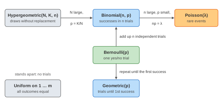
- Bernoulli → binomial. A binomial count is the sum of n independent Bernoulli trials. That is why its mean and variance are n times the Bernoulli ones.
- Bernoulli → geometric. Run the same trials, but ask a different question: not "how many successes" but "how long until the first one".
- Binomial → Poisson. Use many trials with a small p and keep np = λ fixed. The binomial bars slide onto the Poisson bars. See Binomial vs Poisson.
- Hypergeometric → binomial. When the urn is much larger than the sample, taking a ball out hardly changes what is left. The factor (N − n)/(N − 1) goes to 1. With 50 balls, 15 red, draw 5, the variance is already 0.96, close to the binomial 1.05.
Samples and the PMF
A PMF is about the long run. Press Draw 20 samples and the page runs the experiment 20 times with a seeded random generator. Each navy mark shows the share of samples that gave that k. After 20 samples the marks are rough. After 200 they sit close to the bars (Demo: 200 samples approach the PMF). This is the law of large numbers at work: shares of many samples settle on the probabilities.
See also PDF and CDF for running totals of a distribution, Central Limit Theorem for why sums of many samples look like a bell, and Continuous Distributions for the distributions of values that are not whole numbers.
What the page leaves out
- The negative binomial (trials until the r-th success) and the multinomial (more than two outcomes per trial).
- CDFs, P(X ≤ k), and tail probabilities.
- Continuous distributions such as the normal and the exponential.
- The other geometric convention, which counts the failures before the first success (k = 0, 1, 2, …).
- Fitting a distribution to data and testing the fit.