Searching Sorted List Visualization

Searching a sorted list

Given a list of numbers and a value, where in the list is the value, if anywhere? A search returns the index of the value, or -1 if it is not there. This page shows the two basic methods on a sorted list of random numbers between 1 and 999: linear search, which looks at the elements one by one, and binary search, which uses the order to throw away half of the remaining list with every comparison.

Type a whole number into the text field and press Linear Search or Binary Search. Small shows a list of 16 elements, Large a list of 30; switching size makes a new random list. The Searching For box shows the value, the Result box the index found (or -1), with "Element found" or "Element Not found" next to it. The small numbers under the cells are the indices.

Linear search

Start at index 0 and step to the right until you find the value. Because this list is sorted, the page's version can also stop early: as soon as it reaches an element that is not smaller than the value, the value can't appear further to the right.

def linearSearch(listData, value):
    index = 0
    while (index < len(listData) and listData[index] < value):
        index = index + 1
    if (index >= len(listData) or listData[index] != value):
        return -1
    return index

On the canvas the index box and a circle follow the current position. For an unsorted list, drop the early stop and test listData[index] == value instead; then an absent value always costs a pass over the whole list.

Binary search

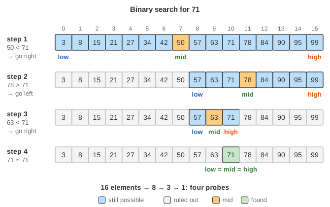
Binary search keeps a range low .. high of indices where the value can still be. It looks at the middle element of that range. If it is the value, done. If it is smaller than the value, the value can only be to its right, so the left half and the middle are discarded; if it is larger, the right half and the middle are discarded. When the range becomes empty (low > high), the value is not in the list.

def binarySearch(listData, value):
    low = 0
    high = len(listData) - 1
    while (low <= high):
        mid = (low + high) // 2          # round down (the canvas writes / 2)
        if (listData[mid] == value):
            return mid
        elif (listData[mid] < value):
            low = mid + 1                # value can only be right of mid
        else:
            high = mid - 1               # value can only be left of mid
    return -1

The canvas shows low in a blue box and circle, mid in green and high in orange. Elements that have been ruled out fade, so you can watch the live range shrink by half each round; they reappear when the search ends.

Worked example

Take this sorted list of 16 elements (the page draws its own random list, but it works the same way):

index   0   1   2   3   4   5   6   7   8   9  10  11  12  13  14  15
value   3   8  15  21  27  34  42  50  57  63  71  78  84  90  95  99

Searching for 71 (present):

low  high  mid  listData[mid]  compare         next range
 0    15    7        50        50 < 71     low  = 8     -> 8..15
 8    15   11        78        78 > 71     high = 10    -> 8..10
 8    10    9        63        63 < 71     low  = 10    -> 10..10
10    10   10        71        equal: return 10

Searching for 40 (absent):

low  high  mid  listData[mid]  compare         next range
 0    15    7        50        50 > 40     high = 6     -> 0..6
 0     6    3        21        21 < 40     low  = 4     -> 4..6
 4     6    5        34        34 < 40     low  = 6     -> 6..6
 6     6    6        42        42 > 40     high = 5     -> 6..5 is empty
low = 6 > high = 5: return -1

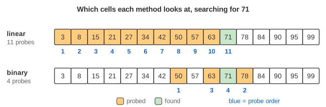
Four probes in each case. Linear search needs 11 comparisons to reach 71 at index 10, and 7 to find that 40 is missing (it stops at 42, index 6). Notice where low ends up in the failed search: 6, exactly the position where 40 would have to be inserted to keep the list sorted (between 34 and 42). That is a useful by-product of binary search.

Why binary search is correct

The key is a loop invariant: if the value is anywhere in the list, it is in listData[low..high]. It holds at the start, when the range is the whole list. In each round, if listData[mid] < value, then because the list is sorted every element at index mid or less is also smaller than the value, so none of them can be it and setting low = mid + 1 keeps the invariant; the case listData[mid] > value is symmetric. Each round makes the range strictly smaller, so the loop ends. It ends either by finding the value, or with an empty range, and then the invariant says the value is nowhere in the list. The invariant depends entirely on the list being sorted.

Running time

• Linear search: O(n) comparisons in the worst case and about n/2 on average for a value that is present.
• Binary search: the range of n elements shrinks to at most half each round, so at most ⌊log₂ n⌋ + 1 probes: 5 for the 16- and 30-element lists here, 10 for a thousand elements, 20 for a million. That is O(log n).
• Both use O(1) extra space; a recursive binary search uses O(log n) stack.
• Sorting first costs O(n log n), so for a single search in unsorted data linear search is the better choice. Binary search pays off when the same list is searched many times.

Common mistakes and edge cases

• Unsorted input: binary search on an unsorted list silently gives wrong answers, often reporting present values as missing.
• Off-by-one in the loop test: with high = len - 1 (an inclusive range) the test must be low <= high. Writing low < high skips the last one-element range; in the search for 71 above it would stop at low = high = 10 without looking at 71.
• Forgetting the ±1: writing low = mid or high = mid with an inclusive range can loop forever once low and high are neighbours, because mid stops moving.
• Overflow in (low + high) / 2: with fixed-size integers (Java, C, C++) the sum can overflow for very large arrays; this bug sat in the Java library for years. Write low + (high - low) / 2 instead. And make sure the division rounds down to a whole index.
• Duplicates: if the value occurs several times, the algorithm returns some matching index, not necessarily the first. To get the first one, keep searching left after a match (the "lower bound" variant).
• Empty list: high = -1, the loop doesn't run and the result is -1, as it should be.

Variants and where it is used

Library functions such as Python's bisect, C++'s std::lower_bound and Java's Arrays.binarySearch are binary searches. The same halving idea is used to search a sorted file or database index (binary search trees and B-trees are binary search turned into a data structure), to find the commit that introduced a bug (git bisect), and to "binary search on the answer" for the smallest value that satisfies a test, such as the smallest capacity that is enough. Interpolation search guesses the position from the values instead of taking the middle, and exponential search first doubles an index to find a range when the list's length is unknown. Linear search remains the right tool for short or unsorted lists and for linked lists, where jumping to the middle isn't possible.

References

Binary search algorithm

Linear search