The idea: plan, move, sense, replan
A robot has to drive from S to G, but its map is not fully right. Cells it has not seen are assumed to be what its map says. It plans a shortest path on that map, takes one step, and looks around with its sensor (every cell within 2 cells). When the sensor, or a map update, shows that the map was wrong, the plan may no longer be valid, so the robot replans. This repeats until it reaches G, or learns that G cannot be reached.
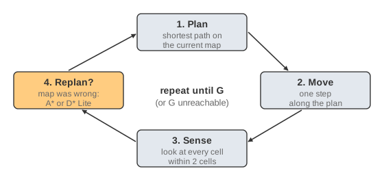
The page runs two planners for the same robot, side by side, at the same time. Each step of a search expands one cell on the left and one cell on the right (or 3 or 10, under Options). The left planner, A*, throws its old search away and searches again from scratch. The right planner, D* Lite, keeps its old search and repairs only the part the change made wrong. Both search backwards, from G to the robot, so the number in a cell means the same thing on both sides: g, the cost from that cell to G.
Two numbers per cell: g and rhs
D* Lite keeps two values for every cell. g(s) is its current estimate of the cost from s to G. rhs(s) is a one-step lookahead: the best neighbour's g plus the cost of the step to it.
A cell is consistent when g = rhs. Only inconsistent cells are in the priority queue U. When the map changes, the costs c(s, s′) of a few steps change, so a few rhs values change, and those cells become inconsistent. D* Lite then works only on them and on what they affect.
| State | Meaning | Colour (right grid) | What D* Lite does when it pops the cell |
|---|---|---|---|
| g = rhs | consistent: g is settled | blue (expanded in this search) or pale blue (kept from an earlier search) | not in the queue |
| g > rhs | overconsistent: a cheaper way to G was found; g will fall | green | g := rhs, then lower the rhs of its neighbours |
| g < rhs | underconsistent: the old way to G got dearer or blocked; g must rise | pink | g := ∞, then recompute the rhs of the neighbours that went through it |
On the left, A* shows the usual open list (green) and closed cells (blue). Inside the queue a cell shows its rhs (the value it is about to get); elsewhere it shows g.
The queue key and km
The queue is ordered by a key of two numbers, compared first by k1, then by k2:
CalculateKey(s) = [ min(g(s), rhs(s)) + h(s_start, s) + km ; min(g(s), rhs(s)) ]
k1 is like A*'s f = g + h, with h the octile distance from the robot (s_start). k2 is like g. A* on the left uses the same order: smallest f, then smallest g, then the cell number. That is why, with no change, D* Lite's first search is exactly a backward A* search, with the same expansions (Demo 1: no change, 69 and 69).
When the robot moves, h changes for every cell, so all keys in the queue are out of date. Re-sorting the queue would cost as much as a new search. Instead, D* Lite adds h(s_last, s_start), the distance the robot moved, to an offset km each time it replans. Old keys are then still lower bounds. When an old key reaches the top, D* Lite recomputes it; if it went up, the cell goes back into the queue with its new key (a re-key, counted separately on the page).
ComputeShortestPath():
  while U.TopKey() < CalculateKey(s_start) or rhs(s_start) > g(s_start):
    u = U.Top();  k_old = U.TopKey();  k_new = CalculateKey(u)
    if k_old < k_new:  U.Update(u, k_new)                  # re-key
    else if g(u) > rhs(u):                                 # overconsistent
      g(u) = rhs(u);  U.Remove(u)
      for s in Pred(u):  rhs(s) = min(rhs(s), c(s,u) + g(u));  UpdateVertex(s)
    else:                                                  # underconsistent
      g_old = g(u);  g(u) = ∞
      for s in Pred(u) ∪ {u}:
        if rhs(s) == c(s,u) + g_old:  rhs(s) = min over s' of c(s,s') + g(s')
        UpdateVertex(s)

after a move, if some edge costs changed:
  km = km + h(s_last, s_start);  s_last = s_start
  for every changed edge (u, v):  fix rhs(u);  UpdateVertex(u)
  ComputeShortestPath()
The search stops as soon as nothing in the queue sorts before the robot's own key and the robot's rhs is not above its g. The robot's cell itself is not expanded; A* on the left stops by the same rule.
When D* Lite saves work, and when it does not
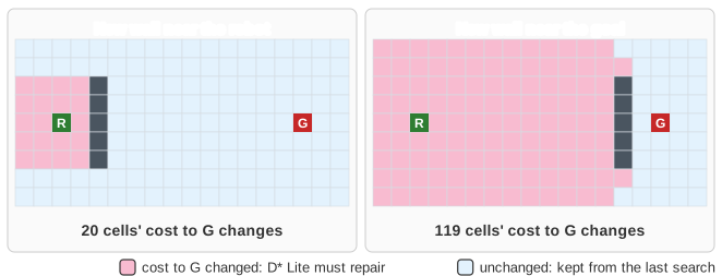
Because D* Lite searches from G, g(s) is the cost from s to G. A change near the robot changes the costs to G of only a few cells, the ones between the change and the robot. A change near G changes the costs to G of almost every cell behind it, and D* Lite must fix each of them.
| Demo | A* (from scratch) | D* Lite | What you see |
|---|---|---|---|
| no change | 69 | 69 | One search each, the same cells in the same order. Path cost 18.49. |
| wall near the robot | 66 + 88 = 154 | 66 + 38 = 104 | After move 1 the sensor finds a wall 2 cells ahead. A* redoes the whole search; D* Lite keeps the g values behind the long wall. |
| wall near the goal | 17 + 45 = 62 | 17 + 58 = 75 (+3 re-keyed) | A map update drops a wall in front of G. Most costs to G go up, so D* Lite has more to repair than a fresh search has to do. |
| several walls over time | 286 in 9 searches | 152 in 9 searches (+47 re-keyed) | Four unseen walls, found piece by piece: 8 replans. Small repairs add up. |
| a wall that is not there | 117 + 60 + 42 = 219 | 117 + 4 + 3 = 124 | The sensor finds an open door in a wall the robot believed was closed. Steps get cheaper, cells turn overconsistent (green), and the robot takes the shortcut (cost 21.83 → 17.66). |
| goal becomes unreachable | 18 + 12 = 30 | 18 + 22 = 40 (+5 re-keyed) | G's door is shut. A* from G runs out of cells at once; D* Lite has to raise every g that went through the door to ∞ before it can say "no path". |
Part of D* Lite's work in a replan is not caused by the change at all: cells left in the queue at the end of the last search (its old frontier) can now sort before the robot's key, so they are expanded too.
Same robot, same moves
Both planners plan for one robot, drawn on both grids. A plan is read the way D* Lite's paper does it: from the robot, step to the neighbour s′ with the smallest c(robot, s′) + g(s′). Ties are broken by a fixed order (up, right, down, left, then the diagonals). Both planners use the same rule on their own g values and the same queue order, so they give the same shortest path, and both robots take the same step. The page checks after every search that both plans are the same path with the same cost (✓ under each grid).
Moves are 8-connected without corner cutting: a diagonal step needs both side cells free. A straight step costs 1, a diagonal step √2. The octile distance never overestimates these costs, so both planners find shortest paths on the known map.
See also Grid Pathfinding Side by Side (two finders racing on a fixed map), Grid Pathfinding (one finder in detail) and A* Search on a general graph.
What the page leaves out
- The heap: both queues here are plain lists scanned for the smallest key. Real implementations use a binary heap, which is what makes re-keys and lazy updates matter for speed.
- Forward A*: re-running A* from the robot towards G works the same way but cannot share cell values with D* Lite; the page uses backward A* so both sides show the cost to G.
- Cheaper A* replanning tricks: replanning only when the plan itself is blocked, or Adaptive A*, which improves h from earlier searches.
- Lifelong Planning A* (LPA*), the algorithm D* Lite is built on: it repairs a search between a fixed start and goal; D* Lite adds km so the start can move.
- Sensor noise, robot size and moving obstacles.