The idea: one loop, different priorities
A game character, a robot or a route planner often moves on a grid. Some cells are walls, some are slow to cross, and the job is to find a path from the start S to the goal G. Every finder on this page runs the same loop:
put S in the open list
while the open list is not empty:
    take the best cell out of the open list and close it
    if it is G: follow the parent pointers back to S, done
    for each neighbour that is not closed:
        if it is new, or this way is cheaper: set its parent, put it in the open list
no path
The finders differ in one thing: what "best" means. The cell text on the canvas is the number the finder sorts by. The panel on the right shows the open list in the order the cells will come out.
| Finder | Takes next | Finds |
|---|---|---|
| Breadth-first search (BFS) | the oldest cell (a queue) | the fewest steps |
| Dijkstra | smallest g, the cost from S | the cheapest path |
| A* | smallest f = g + h | the cheapest path, if h never overestimates |
| Greedy Best-First | smallest h, the estimate to G | some path, often fast, no promise |
| Bidirectional BFS | oldest cell, alternating between a search from S and one from G | the fewest steps, with about half the frontier |
| Jump Point Search | smallest f, but only jump points | the cheapest path on a grid where every cell costs the same |
The grid and its costs
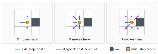
A step to one of the four side neighbours costs 1. A diagonal step costs √2 ≈ 1.41. Stepping into a mud cell costs 5 times as much. The moves option sets the diagonal rule, using the names from PathFinding.js:
- 4, never diagonal: four neighbours.
- 8, no corner cutting (
OnlyWhenNoObstacles): a diagonal step is allowed only when both side cells next to it are free, so a path never squeezes past the corner of a wall. - 8, may cut a corner (
IfAtMostOneObstacle): one of the two side cells may be a wall.
Open and closed cells
A cell is open (green) when it has been discovered but not finished. It is closed (blue) once it has been taken from the open list. The orange cell is the one being expanded now. Counting expansions is a fair way to compare finders, because each one costs about the same work. The panel shows them as expanded. As in PathFinding.js, a closed cell is never reopened. With a good heuristic, it never needs to be.
BFS counts steps, Dijkstra counts cost
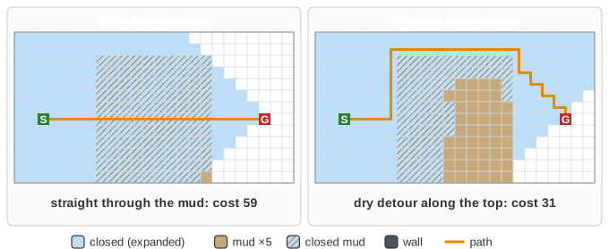
BFS finishes every cell one step away before any cell two steps away. So the first time it reaches G, it has the path with the fewest steps. That is also the cheapest path only when every step costs the same. In the swamp, the straight line through the mud has the fewest steps, so BFS takes it. Dijkstra takes the dry detour, which has more steps but costs much less. Demo: BFS walks through mud; to watch both run at the same time, see Grid Pathfinding Side by Side.
A* and admissible heuristics
A* adds h, an estimate of the cost from a cell to G, so cells that point towards the goal come out first. If h never overestimates the real remaining cost, the heuristic is admissible. Then A* returns the cheapest path. It also expands no more cells than Dijkstra, and usually far fewer. Demos: A* through a gap; Dijkstra, same map, or both at once on Grid Pathfinding Side by Side.
| Heuristic | Formula (dx, dy = distance to G) | Never diagonal | With diagonals |
|---|---|---|---|
| Manhattan | dx + dy | exact without walls, admissible | overestimates: it counts a diagonal step as 2 |
| Euclidean | √(dx² + dy²) | admissible, weak | admissible |
| Octile | max + (√2 − 1)·min | admissible, weak | exact without walls, admissible |
| Chebyshev | max(dx, dy) | admissible, weak | admissible, weak |
A heuristic that is closer to the real cost (without going over) guides the search better. Octile is the best choice when diagonal moves are allowed. Manhattan is the best when they are not. Demo: Manhattan overestimates shows A* losing its guarantee: the path costs 29.49 instead of 27.49, though it expands only 47 cells, against 127 with octile.
Mud is not in the heuristic. The estimates assume every cell is dry, so they stay admissible, but they guide the search less well near mud.
Weighted A* and Greedy Best-First
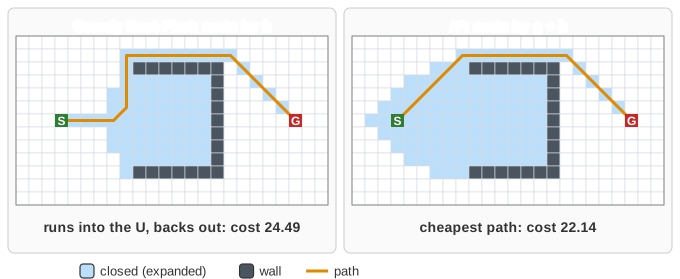
Weighted A* sorts by g + w·h with w > 1. It trusts the estimate more, so it expands fewer cells. The price is a path that can cost up to w times the optimum. Greedy Best-First is the extreme case: it sorts by h alone. In open ground it runs straight at the goal. A dead end shaped like a U, facing the start, traps it: it fills the inside of the U before it backs out. Demos: weighted A* (w = 5); Greedy in a U-trap.
Bidirectional search
Two breadth-first searches take turns, one from S and one from G (pink). Each turn expands one whole layer (every cell at the same depth). When a search reaches a cell the other has already reached, it finishes its layer and keeps the shortest meeting. Stopping at the very first meeting, as PathFinding.js does, can return a path one step too long. Each search only needs to grow to about half the distance. On a large open grid, the area a search covers grows with the square of its radius, so two half-size searches cover about half the area of one full search. On this small grid, the edges and walls limit the saving: on the scattered map BFS expands 253 cells and bidirectional BFS 198. Demo: bidirectional BFS.
When the heuristic cannot help
In a maze the straight-line distance says little about the real distance: the corridor to the goal may first lead away from it. A* still finds the shortest path, but it expands almost as many cells as Dijkstra (60 against 70; Demo: A* in a maze). A heuristic pays off when the map is mostly open.
Jump Point Search
On a grid where every cell costs the same, many paths have equal cost and differ only in the order of their moves. A* opens every one of those cells. Jump Point Search (Harabor and Grastien, 2011) keeps A*'s open list but prunes these symmetric paths. From a cell it keeps moving in a straight line, or diagonally, until something interesting happens. That can be reaching the goal, or a wall ending next to the line, which creates a forced neighbour that the path may need to turn into. Only that cell, a jump point, goes on the open list. The cells passed on the way are scanned (light grey) but never stored. The path is the same as A*'s and just as cheap. Demo: Jump Point Search.
The rules depend on the diagonal mode. The page uses the PathFinding.js versions for "never diagonal" and "no corner cutting". JPS assumes uniform cost, so it ignores mud while searching, and its path through mud is not the cheapest.
When there is no path
A finder can only prove that no path exists by closing every cell it can reach. Demo: no path walls off the only gap, and A* expands the whole left half before it gives up.
See also Grid Pathfinding Side by Side (two finders racing on the same map), A* Search and Dijkstra vs A* on general graphs, Dijkstra's Shortest Path, Breadth-First Search, and the original PathFinding.js demo.
What the page leaves out
- The open list is shown as a sorted list. Real implementations use a binary heap: O(log n) per insert and pop. Ties are broken by smaller h, then by first inserted. Other tie rules give other paths of the same cost.
- IDA* (iterative deepening A*), bidirectional A*/Dijkstra and the "always diagonal" rule from PathFinding.js are not shown.
- Path smoothing, any-angle paths (Theta*), and precomputed methods for large maps (hierarchical A*, contraction hierarchies) are not shown.
- Moving obstacles and replanning (D* Lite, LPA*) are not shown.