The idea: race two finders on the same map
Both grids show the same map. Each runs its own finder, and both run at the same time: every step of the animation expands one cell on the left and one cell on the right. At step k both have done the same amount of work, so the coloured area shows how much each finder had to explore. When one reaches G it draws its path and waits while the other carries on.
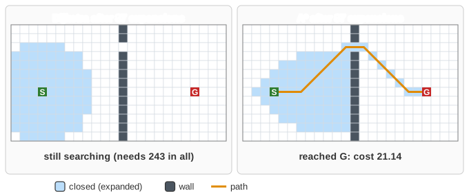
Expanding a cell means taking it out of the open list, closing it (blue) and opening its neighbours (green). The number in a cell is what that finder sorts by, rounded to a whole number. The single-finder page, Grid Pathfinding, shows the full open list and every value with one decimal, and explains each finder in detail.
What to compare
| Demo | What you see |
|---|---|
| Dijkstra vs A* | Same cost (21.14). A* reaches G after 87 expansions. Dijkstra needs 243, growing evenly in every direction. |
| BFS vs Dijkstra in mud | BFS counts steps, so it goes straight through the mud (cost 59). Dijkstra goes around (31). |
| Greedy vs A* in a U-trap | Greedy Best-First goes straight into the U, then has to back out. Its path costs 24.49, against A*'s 22.14. |
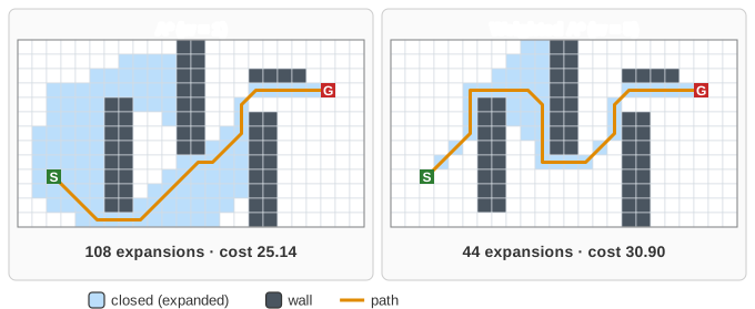
| A* vs weighted A* (w = 5) | Weighted A* trusts the heuristic 5 times more. It expands far fewer cells, but its path costs 30.90 instead of 25.14. |
| octile vs Manhattan | With diagonal moves, Manhattan overestimates. A* with Manhattan finishes after 47 expansions instead of 127, but with cost 29.49 instead of 27.49. |
| BFS vs bidirectional BFS | Two searches, one from S and one from G (pink), meet in the middle: 198 expansions against 253. |
| A* vs Jump Point Search | The same optimal path. JPS opens only the jump points; the cells in between are scanned (grey) but never stored. |
| Dijkstra vs A* in a maze | The straight-line estimate says little in a maze: 60 expansions against 70. |
| no path | The only gap is walled up. Both have to close every reachable cell before they can say there is no path. |
Why count expansions
Each expansion costs every finder about the same work: one open-list removal and up to eight neighbour checks. Comparing after the same number of expansions is therefore fair. Jump Point Search is the exception: its expansions are fewer but each one scans a straight run of cells, so its "scanned" counter is shown too.
What the page leaves out
- Running time in milliseconds: on a 24 × 13 grid every finder takes well under a millisecond.
- The open-list contents, which are on the single-finder page.
- Different moves (diagonal rules) on the two sides: both always use the same rule, so they search the same graph.
See also Grid Pathfinding (one finder, full detail) and Dijkstra vs A* on a general graph.